10 Generalized linear models 10 1 Homogeneous models

10. Generalized linear models • 10. 1 Homogeneous models – Exponential families of distributions, link functions, likelihood estimation • 10. 2 Example: Tort filings • 10. 3 Marginal models and GEE • 10. 4 Random effects models • 10. 5 Fixed effects models – Maximum likelihood, conditional likelihood, Poisson data • 10. 6 Bayesian Inference • Appendix 10 A Exponential families of distributions

10. 1 Homogeneous models • Section Outline – 10. 1. 1 Exponential families of distributions – 10. 1. 2 Link functions – 10. 1. 3 Likelihood estimation • In this section, we consider only independent responses. – No serial correlation. – No random effects that would induce serial correlation.

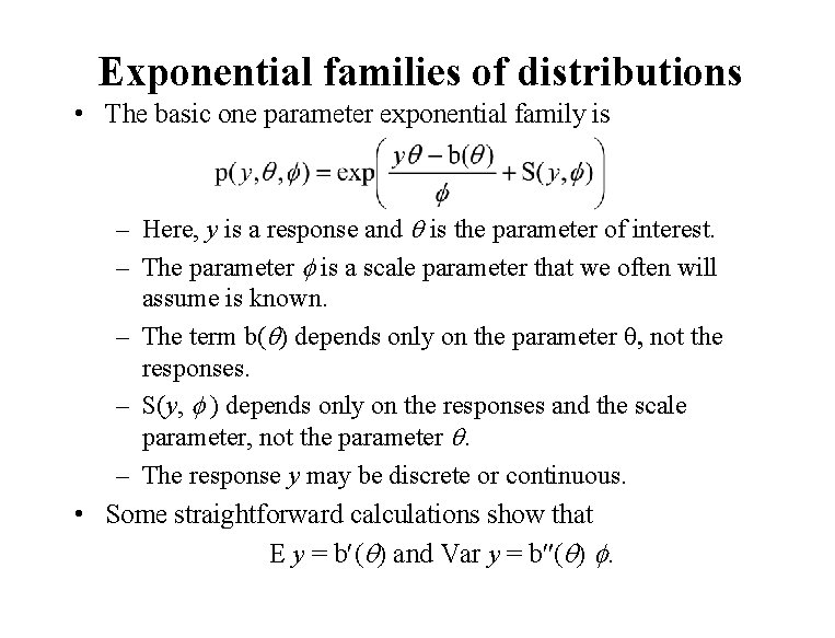
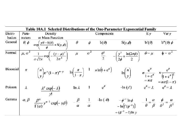
Exponential families of distributions • The basic one parameter exponential family is – Here, y is a response and q is the parameter of interest. – The parameter is a scale parameter that we often will assume is known. – The term b(q) depends only on the parameter q, not the responses. – S(y, ) depends only on the responses and the scale parameter, not the parameter q. – The response y may be discrete or continuous. • Some straightforward calculations show that E y = b (q) and Var y = b (q) .

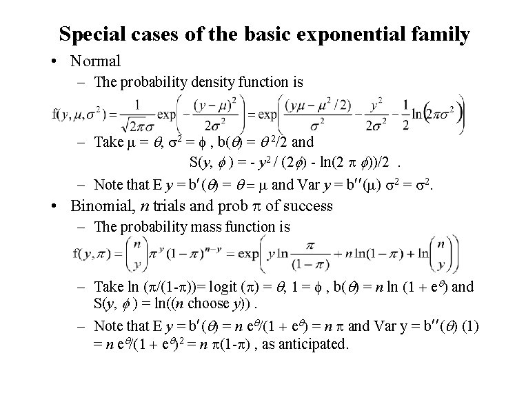
Special cases of the basic exponential family • Normal – The probability density function is – Take m = q, s 2 = f , b(q) = q 2/2 and S(y, ) = - y 2 / (2 ) - ln(2 p ))/2. – Note that E y = b (q) = q = m and Var y = b (m) s 2 = s 2. • Binomial, n trials and prob p of success – The probability mass function is – Take ln (p/(1 -p))= logit (p) = q, 1 = f , b(q) = n ln (1 + eq) and S(y, ) = ln((n choose y)). – Note that E y = b (q) = n eq/(1 + eq) = n p and Var y = b (q) (1) = n eq/(1 + eq)2 = n p(1 -p) , as anticipated.

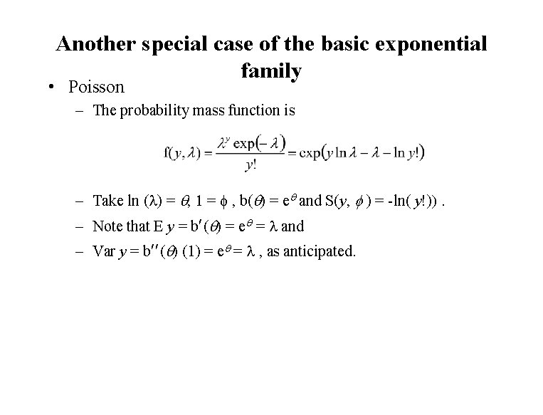
Another special case of the basic exponential family • Poisson – The probability mass function is – Take ln (l) = q, 1 = f , b(q) = eq and S(y, ) = -ln( y!)). – Note that E y = b (q) = eq = l and – Var y = b (q) (1) = eq = l , as anticipated.

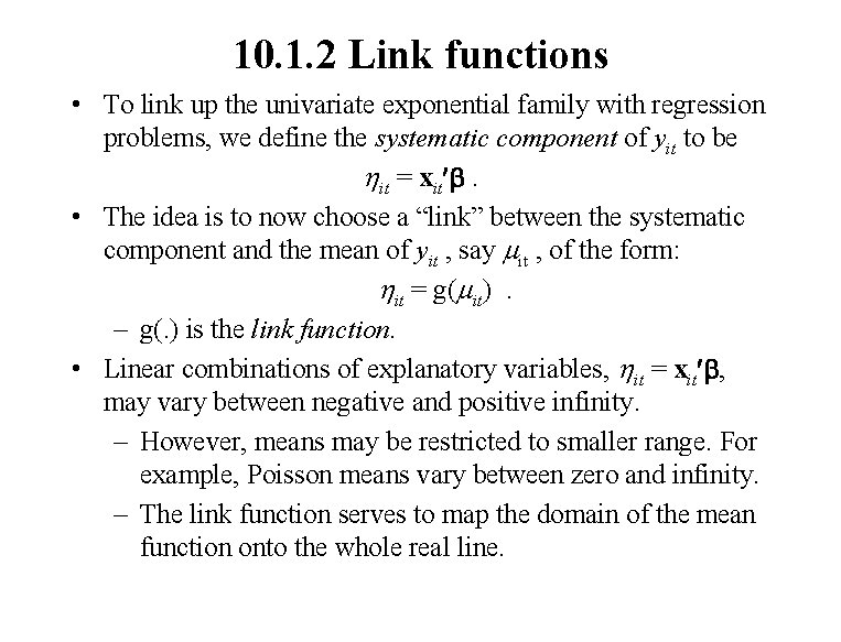
10. 1. 2 Link functions • To link up the univariate exponential family with regression problems, we define the systematic component of yit to be hit = xit b. • The idea is to now choose a “link” between the systematic component and the mean of yit , say mit , of the form: hit = g(mit). – g(. ) is the link function. • Linear combinations of explanatory variables, hit = xit b, may vary between negative and positive infinity. – However, means may be restricted to smaller range. For example, Poisson means vary between zero and infinity. – The link function serves to map the domain of the mean function onto the whole real line.

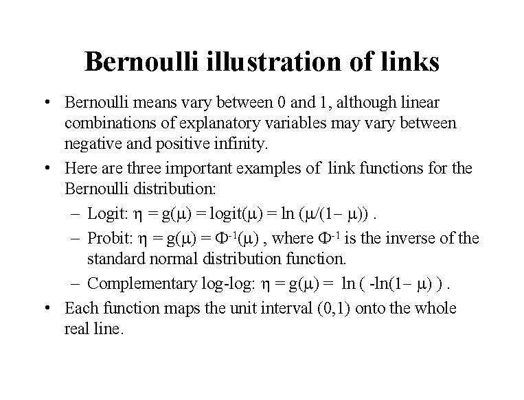
Bernoulli illustration of links • Bernoulli means vary between 0 and 1, although linear combinations of explanatory variables may vary between negative and positive infinity. • Here are three important examples of link functions for the Bernoulli distribution: – Logit: h = g(m) = logit(m) = ln (m/(1 - m)). – Probit: h = g(m) = F-1(m) , where F-1 is the inverse of the standard normal distribution function. – Complementary log-log: h = g(m) = ln ( -ln(1 - m) ). • Each function maps the unit interval (0, 1) onto the whole real line.

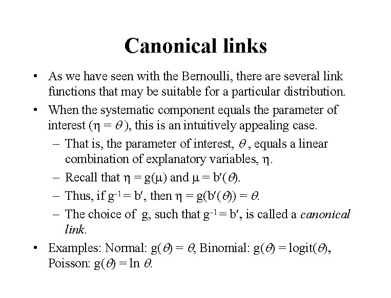
Canonical links • As we have seen with the Bernoulli, there are several link functions that may be suitable for a particular distribution. • When the systematic component equals the parameter of interest (h = q ), this is an intuitively appealing case. – That is, the parameter of interest, q , equals a linear combination of explanatory variables, h. – Recall that h = g(m) and m = b (q). – Thus, if g-1 = b , then h = g(b (q)) = q. – The choice of g, such that g-1 = b , is called a canonical link. • Examples: Normal: g(q) = q, Binomial: g(q) = logit(q), Poisson: g(q) = ln q.

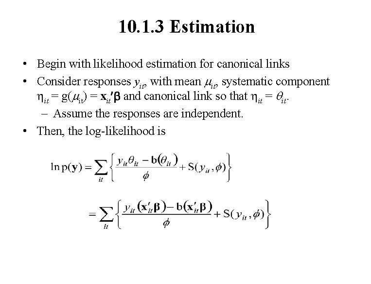
10. 1. 3 Estimation • Begin with likelihood estimation for canonical links • Consider responses yit, with mean mit, systematic component hit = g(mit) = xit b and canonical link so that hit = qit. – Assume the responses are independent. • Then, the log-likelihood is

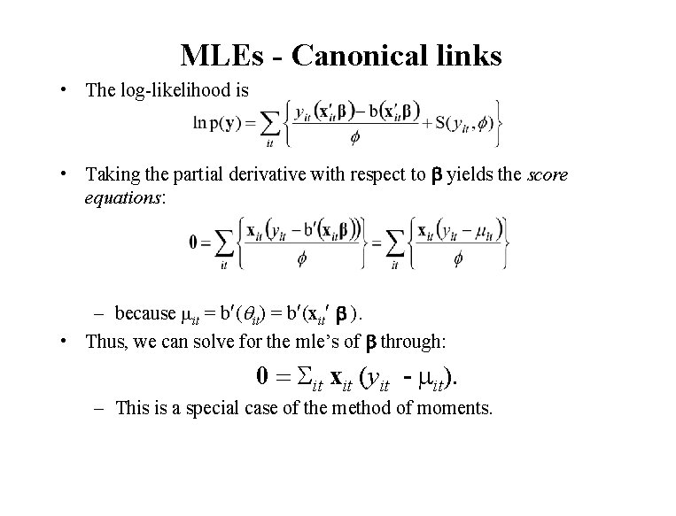
MLEs - Canonical links • The log-likelihood is • Taking the partial derivative with respect to b yields the score equations: – because mit = b (qit) = b (xit b ). • Thus, we can solve for the mle’s of b through: 0 = Sit xit (yit - mit). – This is a special case of the method of moments.

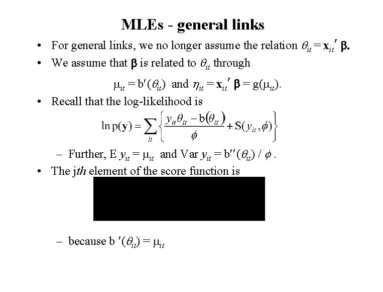
MLEs - general links • For general links, we no longer assume the relation qit = xit b. • We assume that b is related to qit through mit = b (qit) and hit = xit b = g(mit). • Recall that the log-likelihood is – Further, E yit = mit and Var yit = b (qit) / . • The jth element of the score function is – because b (qit) = mit

MLEs - more on general links • To eliminate qit, we use the chain rule to get • Thus, • This yields • This is called the generalized estimating equations form.

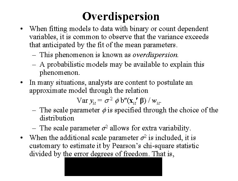
Overdispersion • When fitting models to data with binary or count dependent variables, it is common to observe that the variance exceeds that anticipated by the fit of the mean parameters. – This phenomenon is known as overdispersion. – A probabilistic models may be available to explain this phenomenon. • In many situations, analysts are content to postulate an approximate model through the relation Var yit = 2 b (xit β) / wit. – The scale parameter is specified through the choice of the distribution – The scale parameter σ2 allows for extra variability. • When the additional scale parameter σ2 is included, it is customary to estimate it by Pearson’s chi-square statistic divided by the error degrees of freedom. That is,

10. 2 Example: Tort filings

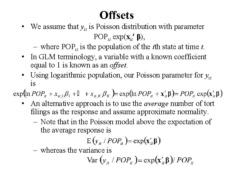
Offsets • We assume that yit is Poisson distribution with parameter POPit exp(xit β), – where POPit is the population of the ith state at time t. • In GLM terminology, a variable with a known coefficient equal to 1 is known as an offset. • Using logarithmic population, our Poisson parameter for yit is • An alternative approach is to use the average number of tort filings as the response and assume approximate normality. – Note that in the Poisson model above the expectation of the average response is – whereas the variance is

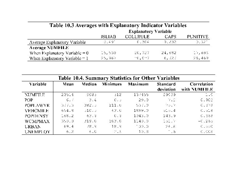
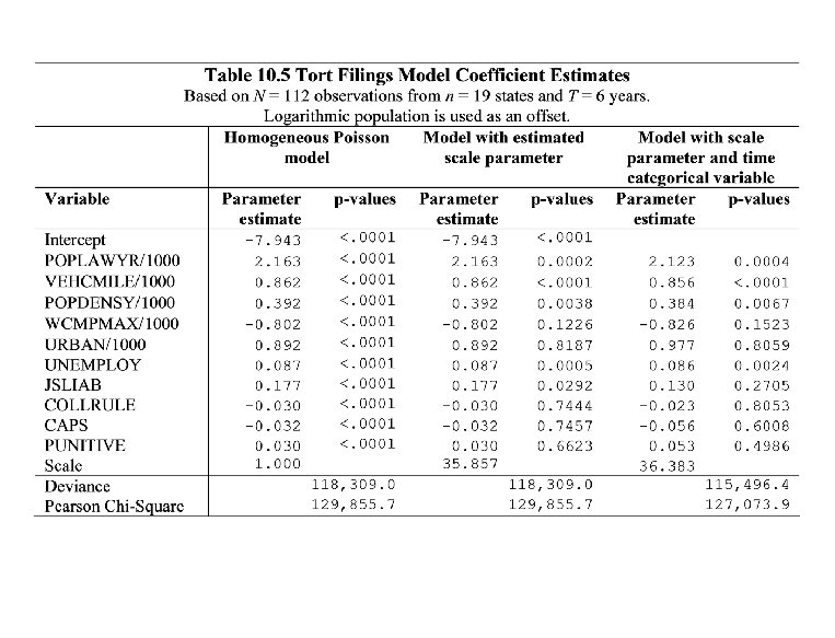
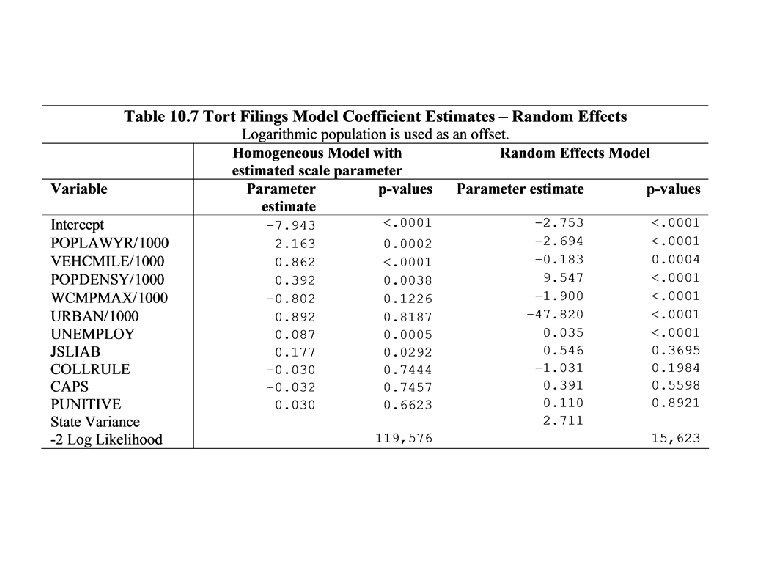
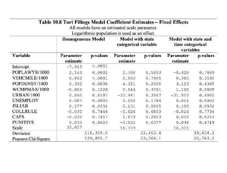
Tort filings • Purpose: to understand ways in which state legal, economic and demographic characteristics affect the number of filings. • Table 10. 3 suggests more filings under JSLIAB and PUNITIVE but less under CAPS • Table 10. 5 – All variables under the homogenous model are statistically significant – However, estimated scale parameter seems important • Here, only JSLIAB is (positively) statistically significant – Time (categorical) variable seems important

10. 3 Marginal models • This approach reduces the reliance on the distributional assumptions by focusing on the first two moments. • We first assume that the variance is a known function of the mean up to a scale parameter, that is, Var yit = v(mit) . – This is a consequence of the exponential family, although now it is a basic assumption. – That is, in the GLM setting, we have Var yit = b (qit) and mit = b (qit). – Because b(. ) and f are assumed known, Var yit is a known function of mit. • We also assume that the correlation between two observations within the same subject is a known function of their means, up to a vector of parameters t. – That is corr(yir , yis ) = r(mir , mis , t) , for r(. ) known.

Marginal model • This framework incorporates the linear model nicely; we simply use a GLM with a normal distribution. – However, for nonlinear situations, a correlation is not always the best way to capture dependencies among observations. • Here is some notation to help see the estimation procedures. • Define mi = (mi 1, mi 2, . . . , mi. Ti)´ to be the vector of means for the ith subject. • To express the variance-covariance matrix, we – define a diagonal matrix of variances Vi = diag(v(mi 1), . . . , v( mi. Ti) ) – and the matrix of correlations Ri(t) to be a matrix with r(mir , mis , t) in the rth row and sth column. – Thus, Var yi = Vi 1/2 Ri(t) Vi 1/2.

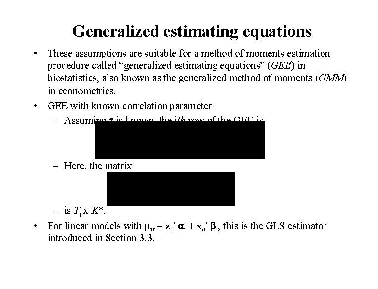
Generalized estimating equations • These assumptions are suitable for a method of moments estimation procedure called “generalized estimating equations” (GEE) in biostatistics, also known as the generalized method of moments (GMM) in econometrics. • GEE with known correlation parameter – Assuming t is known, the jth row of the GEE is – Here, the matrix – is Ti x K*. • For linear models with mit = zit ai + xit b , this is the GLS estimator introduced in Section 3. 3.

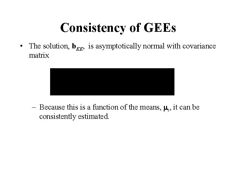
Consistency of GEEs • The solution, b. EE, is asymptotically normal with covariance matrix – Because this is a function of the means, mi, it can be consistently estimated.

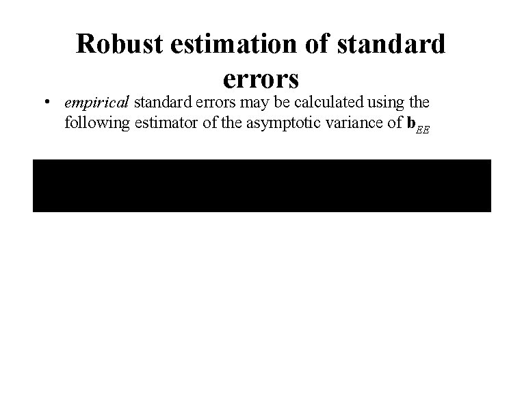
Robust estimation of standard errors • empirical standard errors may be calculated using the following estimator of the asymptotic variance of b. EE

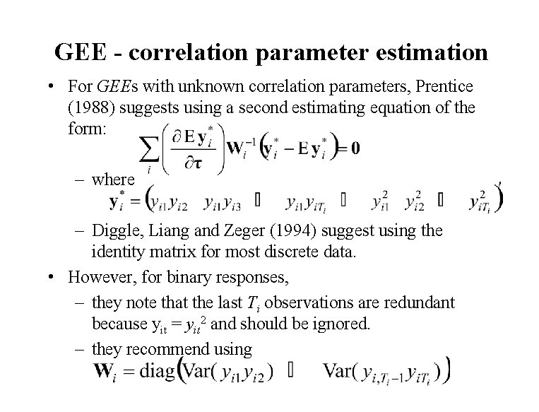
GEE - correlation parameter estimation • For GEEs with unknown correlation parameters, Prentice (1988) suggests using a second estimating equation of the form: – where – Diggle, Liang and Zeger (1994) suggest using the identity matrix for most discrete data. • However, for binary responses, – they note that the last Ti observations are redundant because yit = yit 2 and should be ignored. – they recommend using

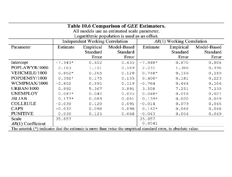
Tort filings • Assume an independent working correlation – This yields at the same parameter estimators as in Table 10. 5, under the homogenous Poisson model with an estimated scale parameter. – JSLIAB is (positively) statistically significant, using both model-based and robust standard errors. • To test the robustness of this model fit, we fit the same model with an AR (1) working correlation. – Again, JSLIAB is (positively) statistically significant. – Interesting that CAPS is now borderline but in the opposite direction suggested by Table 10. 3

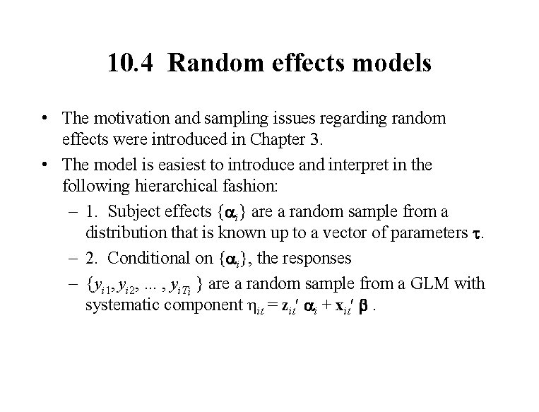
10. 4 Random effects models • The motivation and sampling issues regarding random effects were introduced in Chapter 3. • The model is easiest to introduce and interpret in the following hierarchical fashion: – 1. Subject effects {ai} are a random sample from a distribution that is known up to a vector of parameters t. – 2. Conditional on {ai}, the responses – {yi 1, yi 2, . . . , yi. Ti } are a random sample from a GLM with systematic component hit = zit ai + xit b.

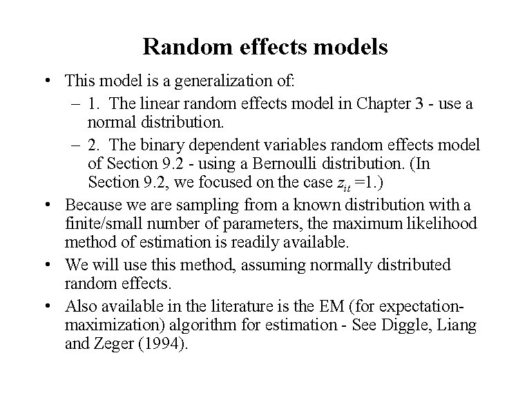
Random effects models • This model is a generalization of: – 1. The linear random effects model in Chapter 3 - use a normal distribution. – 2. The binary dependent variables random effects model of Section 9. 2 - using a Bernoulli distribution. (In Section 9. 2, we focused on the case zit =1. ) • Because we are sampling from a known distribution with a finite/small number of parameters, the maximum likelihood method of estimation is readily available. • We will use this method, assuming normally distributed random effects. • Also available in the literature is the EM (for expectationmaximization) algorithm for estimation - See Diggle, Liang and Zeger (1994).

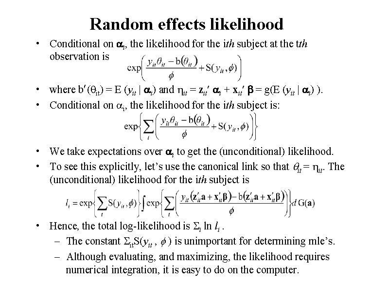
Random effects likelihood • Conditional on ai, the likelihood for the ith subject at the tth observation is • where b (qit) = E (yit | ai) and hit = zit ai + xit b = g(E (yit | ai) ). • Conditional on ai, the likelihood for the ith subject is: • We take expectations over ai to get the (unconditional) likelihood. • To see this explicitly, let’s use the canonical link so that qit = hit. The (unconditional) likelihood for the ith subject is • Hence, the total log-likelihood is Si ln li. – The constant Sit. S(yit , ) is unimportant for determining mle’s. – Although evaluating, and maximizing, the likelihood requires numerical integration, it is easy to do on the computer.

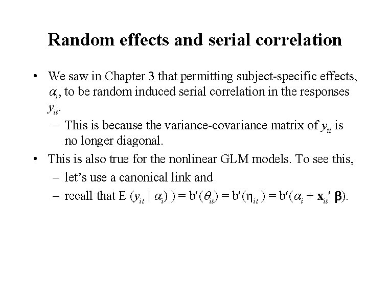
Random effects and serial correlation • We saw in Chapter 3 that permitting subject-specific effects, ai, to be random induced serial correlation in the responses yit. – This is because the variance-covariance matrix of yit is no longer diagonal. • This is also true for the nonlinear GLM models. To see this, – let’s use a canonical link and – recall that E (yit | ai) ) = b (qit) = b (hit ) = b (ai + xit b).

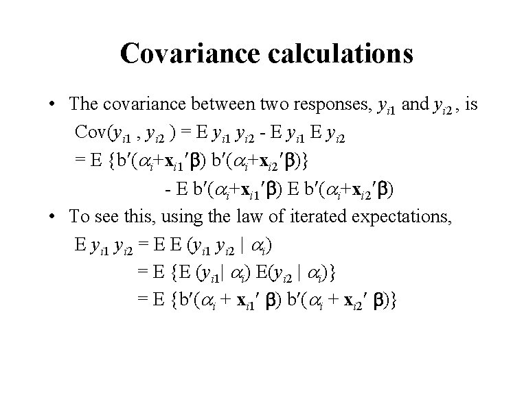
Covariance calculations • The covariance between two responses, yi 1 and yi 2 , is Cov(yi 1 , yi 2 ) = E yi 1 yi 2 - E yi 1 E yi 2 = E {b (ai+xi 1 b) b (ai+xi 2 b)} - E b (ai+xi 1 b) E b (ai+xi 2 b) • To see this, using the law of iterated expectations, E yi 1 yi 2 = E E (yi 1 yi 2 | ai) = E {E (yi 1| ai) E(yi 2 | ai)} = E {b (ai + xi 1 b) b (ai + xi 2 b)}

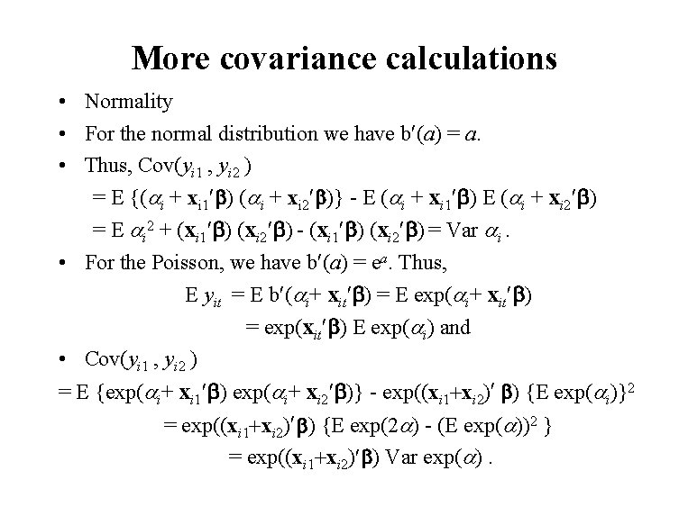
More covariance calculations • Normality • For the normal distribution we have b (a) = a. • Thus, Cov(yi 1 , yi 2 ) = E {(ai + xi 1 b) (ai + xi 2 b)} - E (ai + xi 1 b) E (ai + xi 2 b) = E ai 2 + (xi 1 b) (xi 2 b) - (xi 1 b) (xi 2 b) = Var ai. • For the Poisson, we have b (a) = ea. Thus, E yit = E b (ai+ xit b) = E exp(ai+ xit b) = exp(xit b) E exp(ai) and • Cov(yi 1 , yi 2 ) = E {exp(ai+ xi 1 b) exp(ai+ xi 2 b)} - exp((xi 1+xi 2) b) {E exp(ai)}2 = exp((xi 1+xi 2) b) {E exp(2 a) - (E exp(a))2 } = exp((xi 1+xi 2) b) Var exp(a).

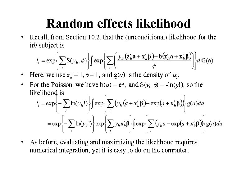
Random effects likelihood • Recall, from Section 10. 2, that the (unconditional) likelihood for the ith subject is • Here, we use zit = 1, and g(a) is the density of ai. • For the Poisson, we have b(a) = ea , and S(y, ) = -ln(y!), so the likelihood is • As before, evaluating and maximizing the likelihood requires numerical integration, yet it is easy to do on the computer.

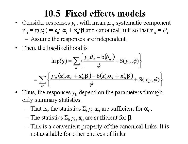
10. 5 Fixed effects models • Consider responses yit, with mean mit, systematic component hit = g(mit) = zit ai + xit b and canonical link so that hit = qit. – Assume the responses are independent. • Then, the log-likelihood is • Thus, the responses yit depend on the parameters through only summary statistics. – That is, the statistics St yit zit are sufficient for ai. – The statistics Sit yit xit are sufficient for b. – This is a convenient property of the canonical links. It is not available for other choices of links.

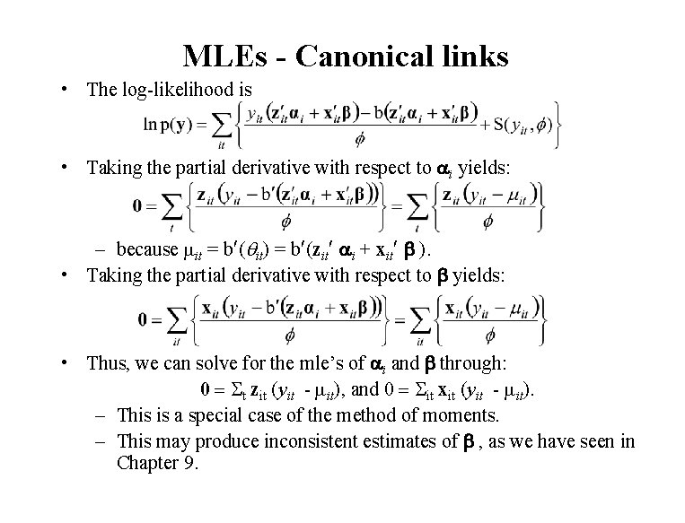
MLEs - Canonical links • The log-likelihood is • Taking the partial derivative with respect to ai yields: – because mit = b (qit) = b (zit ai + xit b ). • Taking the partial derivative with respect to b yields: • Thus, we can solve for the mle’s of ai and b through: 0 = St zit (yit - mit), and 0 = Sit xit (yit - mit). – This is a special case of the method of moments. – This may produce inconsistent estimates of b , as we have seen in Chapter 9.

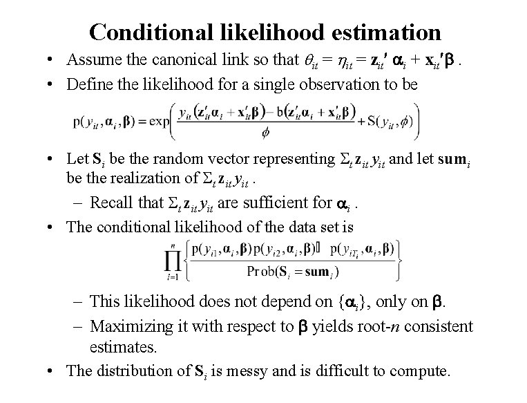
Conditional likelihood estimation • Assume the canonical link so that qit = hit = zit ai + xit b. • Define the likelihood for a single observation to be • Let Si be the random vector representing St zit yit and let sumi be the realization of St zit yit. – Recall that St zit yit are sufficient for ai. • The conditional likelihood of the data set is – This likelihood does not depend on {ai}, only on b. – Maximizing it with respect to b yields root-n consistent estimates. • The distribution of Si is messy and is difficult to compute.

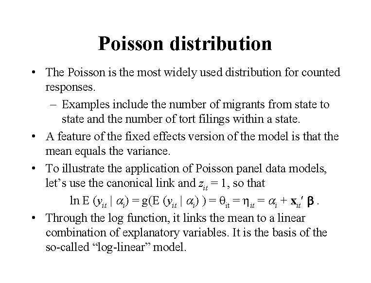
Poisson distribution • The Poisson is the most widely used distribution for counted responses. – Examples include the number of migrants from state to state and the number of tort filings within a state. • A feature of the fixed effects version of the model is that the mean equals the variance. • To illustrate the application of Poisson panel data models, let’s use the canonical link and zit = 1, so that ln E (yit | ai) = g(E (yit | ai) ) = qit = hit = ai + xit b. • Through the log function, it links the mean to a linear combination of explanatory variables. It is the basis of the so-called “log-linear” model.

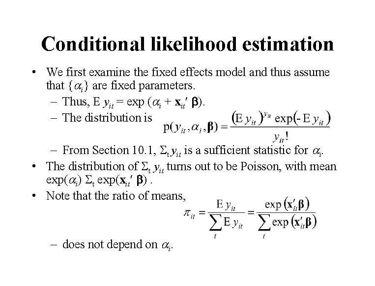
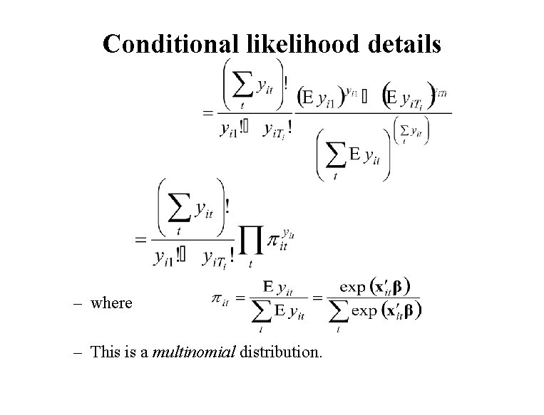
Conditional likelihood estimation • We first examine the fixed effects model and thus assume that {ai} are fixed parameters. – Thus, E yit = exp (ai + xit b). – The distribution is – From Section 10. 1, St yit is a sufficient statistic for ai. • The distribution of St yit turns out to be Poisson, with mean exp(ai) St exp(xit b). • Note that the ratio of means, – does not depend on ai.

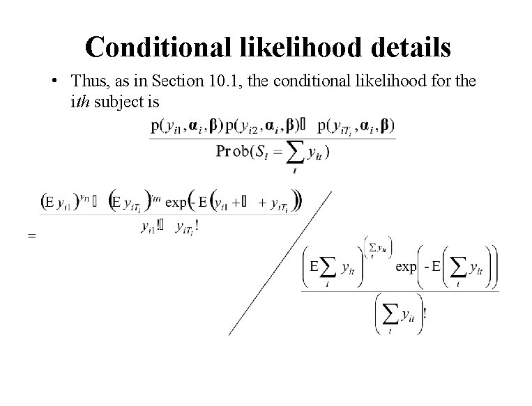
Conditional likelihood details • Thus, as in Section 10. 1, the conditional likelihood for the ith subject is

Conditional likelihood details – where – This is a multinomial distribution.

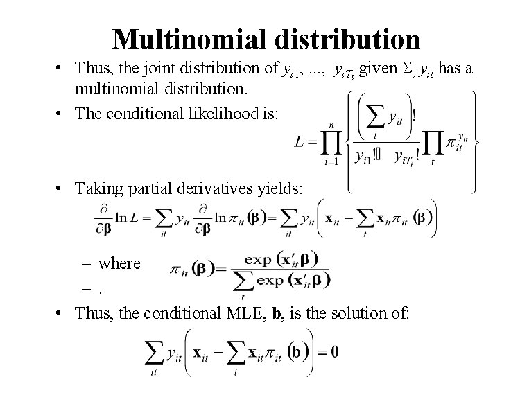
Multinomial distribution • Thus, the joint distribution of yi 1, . . . , yi. Ti given St yit has a multinomial distribution. • The conditional likelihood is: • Taking partial derivatives yields: – where –. • Thus, the conditional MLE, b, is the solution of: