Lecture 11 Chapter 9 Generalized Linear Mixed Models

Lecture 11 (Chapter 9)

Generalized Linear Mixed Models with Random Effects • The logistic regression model with random intercept – Example: 2 x 2 crossover trial – Example: Indonesian Children’s Health Study • The Poisson regression model with random intercept – Example: seizure data

Random Effects GLM • Basic idea: There is natural heterogeneity among subjects. • Systematic part • Random part

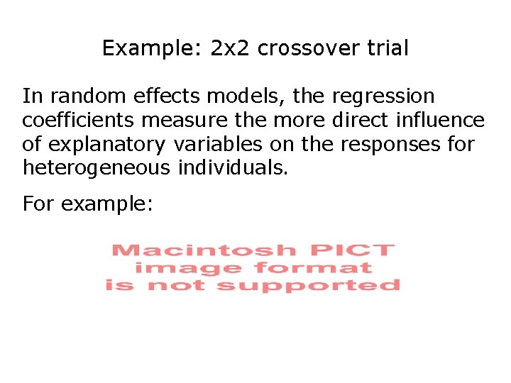
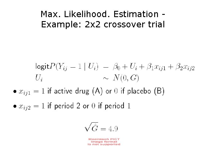
Example: 2 x 2 crossover trial In random effects models, the regression coefficients measure the more direct influence of explanatory variables on the responses for heterogeneous individuals. For example:

Example: 2 x 2 crossover trial (Recall) Example: This model states that: 1. each person has his/her own probability of positive response under a placebo (B)

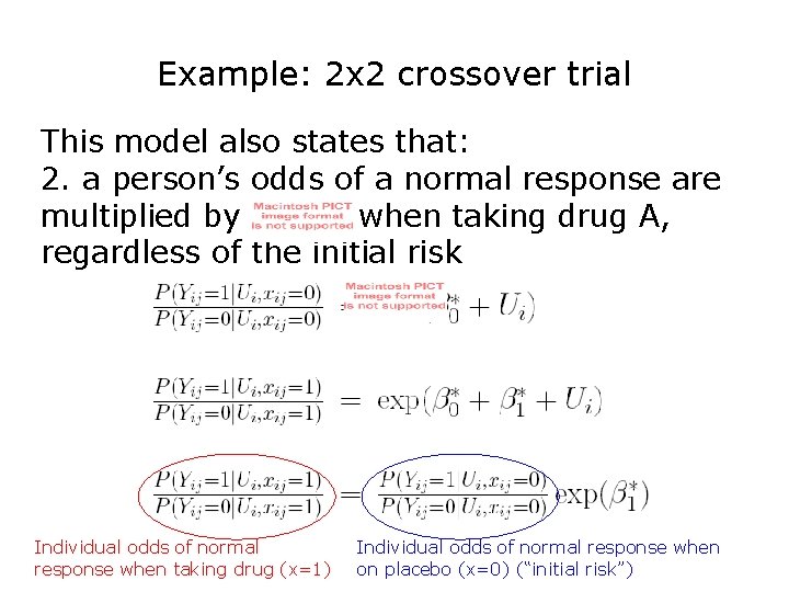
Example: 2 x 2 crossover trial This model also states that: 2. a person’s odds of a normal response are multiplied by when taking drug A, regardless of the initial risk Individual odds of normal response when taking drug (x=1) Individual odds of normal response when on placebo (x=0) (“initial risk”)

In Logistic Models In other words: • Marginal model estimates are smaller than random effects model estimates • Tests of hypotheses approximately the same in random effects as in marginal

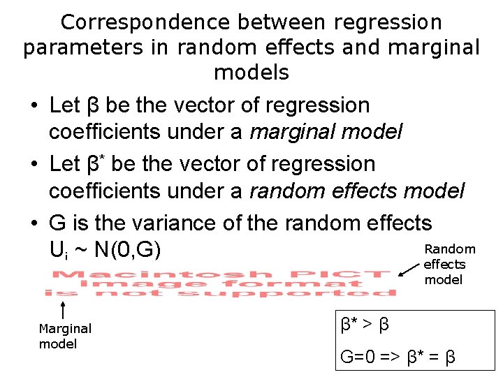
Correspondence between regression parameters in random effects and marginal models • Let β be the vector of regression coefficients under a marginal model • Let β* be the vector of regression coefficients under a random effects model • G is the variance of the random effects Random Ui ~ N(0, G) effects model Marginal model β* > β G=0 => β* = β

Estimation of Generalized Linear Mixed Models • Setting: – f(Yij|Ui) in the exponential family – Yi 1, …, Yini | Ui are independent – Ui ~ f(Ui, G) • Maximum Likelihood Estimation • Ui is a set of unobserved variables which we integrate out of the likelihood

Maximum Likelihood Estimation of G and β • Assume: Ui ~ N(0, G) • We can learn about one individual’s coefficients by understanding the variability in coefficients across the population (G)

Maximum Likelihood Estimation of G and β (cont’d) • If Gi is small, then rely on population average coefficients to estimate those for an individuals – We weight the cross-sectional information more heavily and we borrow strength across subjects • If Gi is large, then rely heavily on the data from each individual to estimate their own coefficients – We weight the longitudinal information more heavily since comparisons within a subject are likely to be more precise than comparisons among subjects

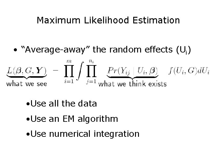
Maximum Likelihood Estimation • “Average-away” the random effects (Ui) • Use all the data • Use an EM algorithm • Use numerical integration

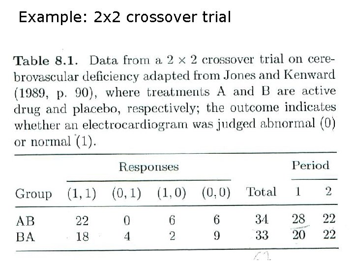
Example: 2 x 2 crossover trial

Max. Likelihood. Estimation Example: 2 x 2 crossover trial

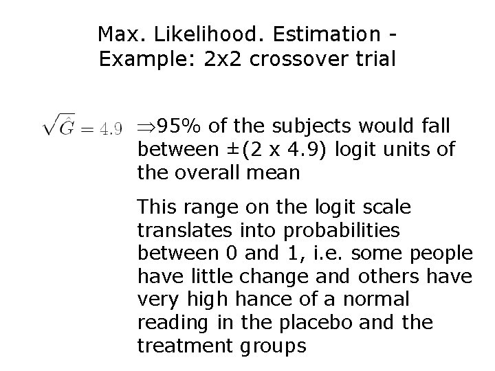
Max. Likelihood. Estimation Example: 2 x 2 crossover trial Þ 95% of the subjects would fall between ±(2 x 4. 9) logit units of the overall mean This range on the logit scale translates into probabilities between 0 and 1, i. e. some people have little change and others have very high hance of a normal reading in the placebo and the treatment groups

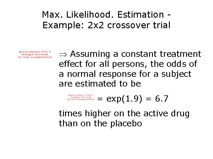
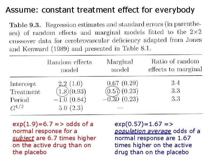
Max. Likelihood. Estimation Example: 2 x 2 crossover trial Þ Assuming a constant treatment effect for all persons, the odds of a normal response for a subject are estimated to be = exp(1. 9) = 6. 7 times higher on the active drug than on the placebo

*robust SE **model-based SE

Assume: constant treatment effect for everybody exp(1. 9)=6. 7 => odds of a normal response for a subject are 6. 7 times higher on the active drug than on the placebo exp(0. 57)=1. 67 => population average odds of a normal response are 1. 67 times higher on the active drug than on the placebo

Example: 2 x 2 crossover trial Summary • Marginal model • Random effects model (maximum likelihood) • The smaller value from the marginal analysis is consistent with theoretical inequality:

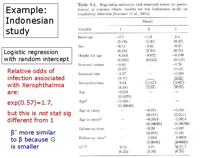
Example: Indonesian study Logistic regression with random intercept Relative odds of infection associated with Xerophthalmia are: exp(0. 57)=1. 7, but this is not stat sig different from 1 β* more similar to β because G is smaller

Indonesian Study: Maximum Likelihood Approach With a random effects model, we can address the question of how an individual child’s risk for respiratory infection will change if his/her vitamin A status were to change. • We assume that each child has a distinct intercept which represents his/her propensity to infection. • We account for correlation by including random intercepts, Ui ~ N(0, G).

Indonesian Study: Maximum Likelihood Approach (cont’d) Þ considerable heterogeneity among children • Among children with linear predictor equal to the intercept (-2. 2), i. e. children of average and height, who are female, and who are vitamin A sufficient, about 95% would have a probability of infection between (0. 025) and (0. 31): • Relative odds of infection associated with vitamin A deficiency are exp(0. 54)=1. 7

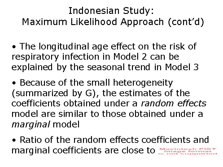
Indonesian Study: Maximum Likelihood Approach (cont’d) • The longitudinal age effect on the risk of respiratory infection in Model 2 can be explained by the seasonal trend in Model 3 • Because of the small heterogeneity (summarized by G), the estimates of the coefficients obtained under a random effects model are similar to those obtained under a marginal model • Ratio of the random effects coefficients and marginal coefficients are close to

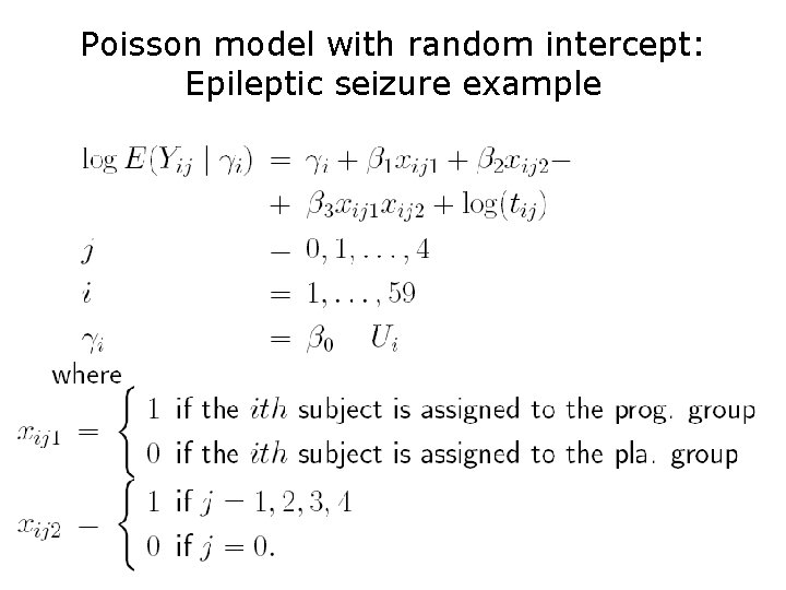
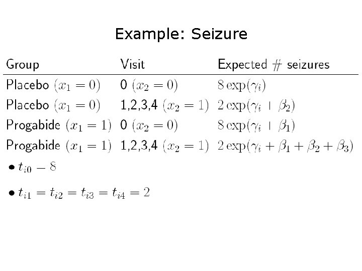
Poisson model with random intercept: Epileptic seizure example

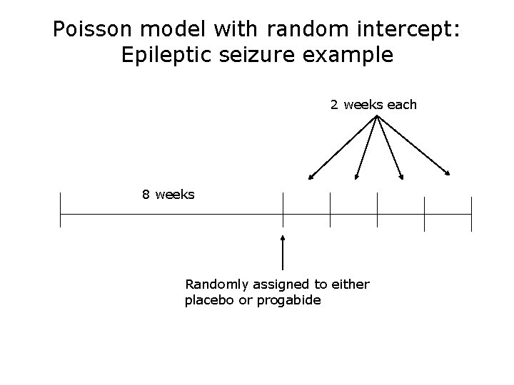
Poisson model with random intercept: Epileptic seizure example 2 weeks each 8 weeks Randomly assigned to either placebo or progabide

Example: Seizure

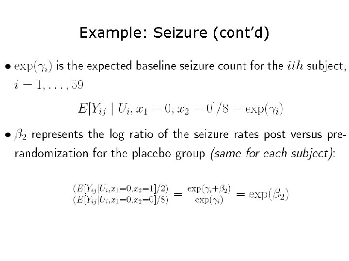
Example: Seizure (cont’d)

Example: Seizure (cont’d)

Example: Seizure (cont’d)

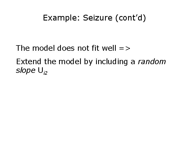
Example: Seizure (cont’d) The model does not fit well => Extend the model by including a random slope Ui 2

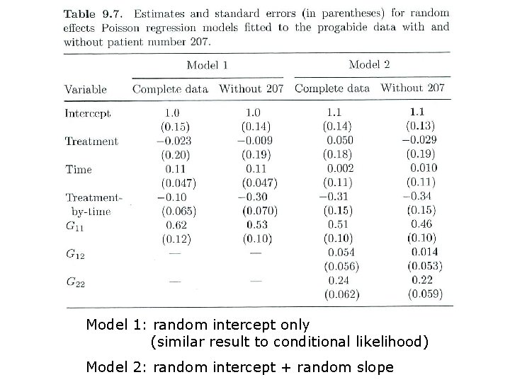
Model 1: random intercept only (similar result to conditional likelihood) Model 2: random intercept + random slope

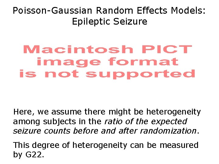
Poisson-Gaussian Random Effects Models: Epileptic Seizure Here, we assume there might be heterogeneity among subjects in the ratio of the expected seizure counts before and after randomization. This degree of heterogeneity can be measured by G 22.

Poisson-Gaussian Random Effects Models: Epileptic Seizure We use maximum likelihood estimation.

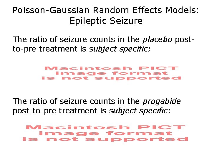
Poisson-Gaussian Random Effects Models: Epileptic Seizure The ratio of seizure counts in the placebo postto-pre treatment is subject specific: The ratio of seizure counts in the progabide post-to-pre treatment is subject specific:

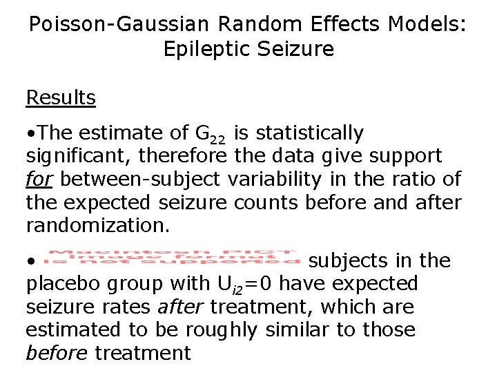
Poisson-Gaussian Random Effects Models: Epileptic Seizure Results • The estimate of G 22 is statistically significant, therefore the data give support for between-subject variability in the ratio of the expected seizure counts before and after randomization. • subjects in the placebo group with Ui 2=0 have expected seizure rates after treatment, which are estimated to be roughly similar to those before treatment

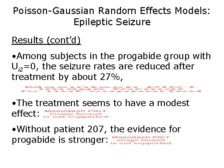
Poisson-Gaussian Random Effects Models: Epileptic Seizure Results (cont’d) • Among subjects in the progabide group with Ui 2=0, the seizure rates are reduced after treatment by about 27%, • The treatment seems to have a modest effect: • Without patient 207, the evidence for progabide is stronger: