Generalized Linear Models on Large Data Sets Joseph

Generalized Linear Models on Large Data Sets Joseph B. Rickert Data Scientist, Community Manager Susan Ranney, Ph. D. Chief Data Scientist, Revolution Analytics BARUG August 12, 2014 Use. R! 2014

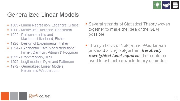
Generalized Linear Models § 1805 - Linear Regression: Legendre, Gauss § 1908 - Maximum Likelihood, Edgeworth § 1922 - Poisson models and Maximum Likelihood, Fisher § 1926 - Design of Experiments, Fisher § 1934 - Exponential Family of distributions Fisher, Darmois, Pitman & Koopman § 1935 - Probit models, Bliss § 1952 - Logit models, Dyke and Patterson § 1972 - Generalized Linear Models, Nelder and Wedderburn § Several strands of Statistical Theory woven together to make the idea of the GLM possible § The synthesis of Nelder and Wedderburn provided a single algorithm, Iteratively reweighted least squares, that could be used to estimate a whole family of models 2

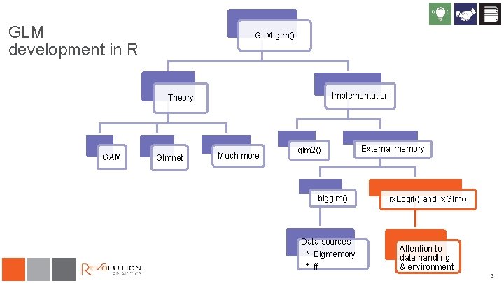
GLM development in R GLM glm() Implementation Theory GAM Glmnet Much more glm 2() bigglm() Data sources * Bigmemory * ff External memory rx. Logit() and rx. Glm() Attention to data handling & environment 3

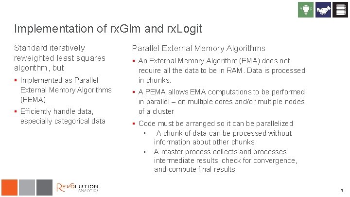
Implementation of rx. Glm and rx. Logit Standard iteratively reweighted least squares algorithm, but § Implemented as Parallel External Memory Algorithms (PEMA) § Efficiently handle data, especially categorical data Parallel External Memory Algorithms § An External Memory Algorithm (EMA) does not require all the data to be in RAM. Data is processed in chunks. § A PEMA allows EMA computations to be performed in parallel – on multiple cores and/or multiple nodes of a cluster § Code must be arranged so it can be parallelized § A chunk of data can be processed without information about other chunks § A master process collects and processes intermediate results, check for convergence, and compute final results 4

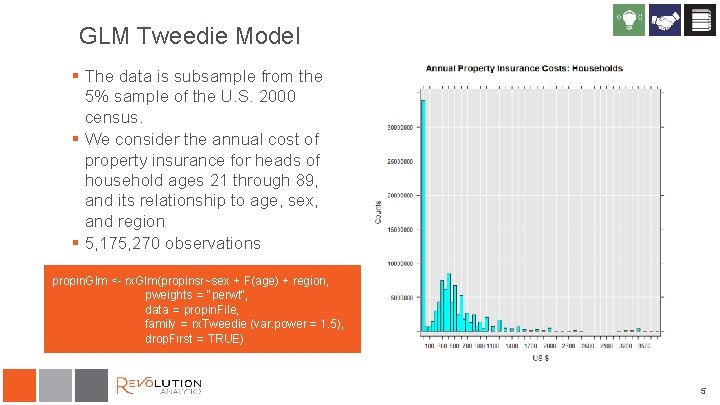
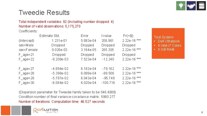
GLM Tweedie Model § The data is subsample from the 5% sample of the U. S. 2000 census. § We consider the annual cost of property insurance for heads of household ages 21 through 89, and its relationship to age, sex, and region § 5, 175, 270 observations propin. Glm <- rx. Glm(propinsr~sex + F(age) + region, pweights = "perwt", data = propin. File, family = rx. Tweedie (var. power = 1. 5), drop. First = TRUE) 5

Tweedie Results Total independent variables: 82 (Including number dropped: 4) Number of valid observations: 5, 175, 270 Coefficients: Estimate Std. Error t value (Intercept) 1. 231 e-01 5. 893 e-04 208. 961 sex=Male Dropped sex=Female 9. 026 e-03 3. 164 e-05 285. 305 F_age=21 Dropped F_age=22 -9. 208 e-03 7. 523 e-04 -12. 240 Pr(>|t|) 2. 22 e-16 *** Dropped 2. 22 e-16 *** F_age=27 F_age=28 F_age=29 F_age=30 2. 22 e-16 *** -4. 894 e-02 6. 182 e-04 -79. 162 -5. 398 e-02 6. 099 e-04 -88. 506 -5. 787 e-02 6. 043 e-04 -95. 749 -6. 064 e-02 6. 020 e-04 -100. 716. . . (Dispersion parameter for Tweedie family taken to be 546. 4888) Condition number of final variance-covariance matrix: 5980. 277 Number of iterations: Computation time: 46. 527 seconds Test System • Dell Ultrabook • 4 Intel i 7 Cores • 8 GB RAM 6

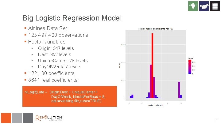
Big Logistic Regression Model § Airlines Data Set § 123, 497, 420 observations § Factor variables § § Origin: 347 levels Dest: 352 levels Unique. Carrier: 29 levels Day. Of. Week: 7 levels § 122, 180 coefficients § 8641 real coefficients rx. Logit(Late ~ Origin: Dest + Unique. Carrier + Day. Of. Week, blocks. Per. Read = 8, data=working. file, cube=TRUE) 7

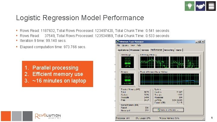
Logistic Regression Model Performance § Rows Read: 1187632, Total Rows Processed: 123497420, Total Chunk Time: 0. 541 seconds § Rows Read: 37549, Total Rows Processed: 123534969, Total Chunk Time: 0. 533 seconds § Iteration 9 time: 99. 140 secs. § Elapsed computation time: 973. 766 secs. 1. Parallel processing 2. Efficient memory use 3. ~16 minutes on laptop 8

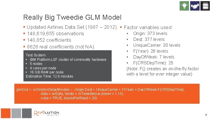
Really Big Tweedie GLM Model § § Updated Airlines Data Set (1987 – 2012) § Factor variables used: § Origin: 373 levels 148, 619, 655 observations § Dest: 377 levels 140, 852 coefficients § Unique. Carrier: 30 levels 8626 real coefficients (not NA) Test System • IBM Platform LSF cluster of commodity hardware • 5 nodes • 4 cores per node • 16 GB RAM per node Estimation Time: 12. 6 minutes F(Year): 26 levels § Day. Of. Week: 7 levels § F(CRSDep. Time): 25 (Note: F() creates an on-the-fly factor with a level for ever integer value) § glm. Out <- rx. Glm(Arr. Delay. Minutes ~ Origin: Dest + Unique. Carrier + F(Year) + Day. Of. Week: F(CRSDep. Time), data = air. Data, family = rx. Tweedie(var. power = 1. 15), cube = TRUE, blocks. Per. Read = 20) 9

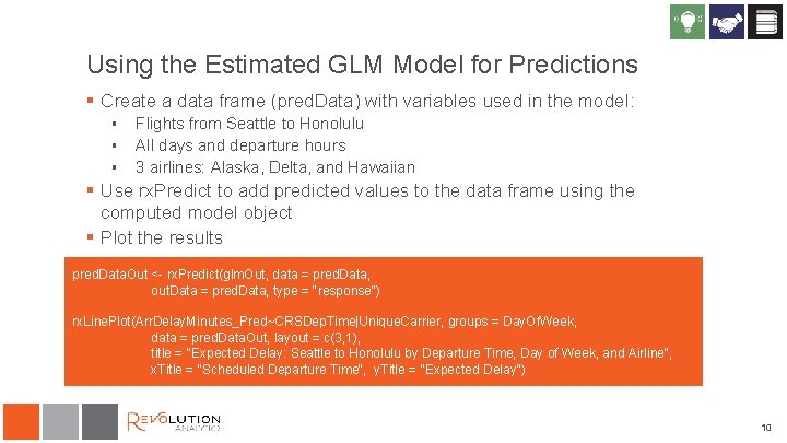
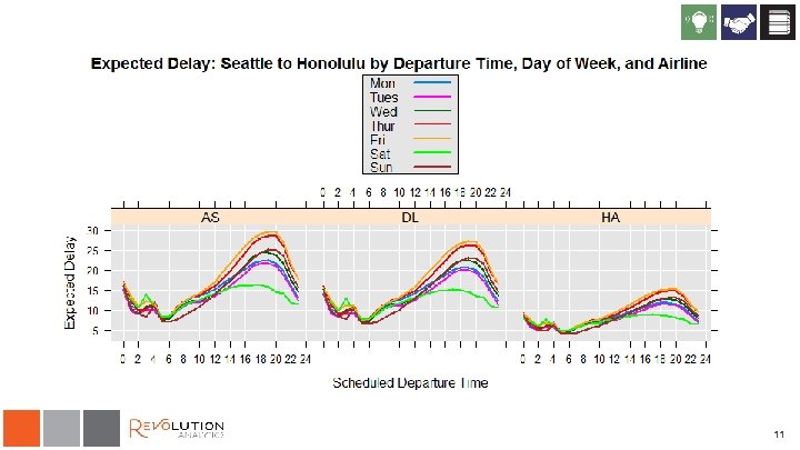
Using the Estimated GLM Model for Predictions § Create a data frame (pred. Data) with variables used in the model: § § § Flights from Seattle to Honolulu All days and departure hours 3 airlines: Alaska, Delta, and Hawaiian § Use rx. Predict to add predicted values to the data frame using the computed model object § Plot the results pred. Data. Out <- rx. Predict(glm. Out, data = pred. Data, out. Data = pred. Data, type = "response") rx. Line. Plot(Arr. Delay. Minutes_Pred~CRSDep. Time|Unique. Carrier, groups = Day. Of. Week, data = pred. Data. Out, layout = c(3, 1), title = "Expected Delay: Seattle to Honolulu by Departure Time, Day of Week, and Airline", x. Title = "Scheduled Departure Time", y. Title = "Expected Delay") 10

11

Summary § The pre-history of the GLM is very rich and includes much fundamental statistical theory. § Nelder and Wedderburn’s 1972 paper synthesized the idea of the GLM, and sparked research both in theory and algorithms § IRLS, the original method of estimating GLMs has proved to be remarkably effective § Good performance on large data sets can be achieved with: § The implementation of parallel code and distributed computing § Careful data handling § Attention to processing factors 12

Some References § § § Bliss, C. J. (1935) The calculation of the dosage-mortality curve Ann. Appl. Biol. 22, 307 -30 Chambers, J. M. (1971) Regression Updating J. ASA Vol 66, Issue 336 Darmois (1935) Sur les lois de probabilité à estimation exhaustive, C. R. Acad. Sci. 200, 1265 -1266 Dyke G. V. , Patterson H. D. (1952) Analysis of factorial arrangements when the data are proportions Biometrics 8: 1– 12 Edgeworth F. Y. (1908) On the probable errors of frequency-constants J. Roy. Statist. Soc. 71 381 – 97, 499 -512, 651 -78 Fisher, R. A. – (1922) On the mathematical foundations of theoretical statistics. Phil Trans. R. Soc 222; 309 -68 – (1934) Two new properties of mathematical likelihood Proc. Roy. Soc. , A. 144, 285 -307 – (1958) Statistical Methods for Research Workers, Oliver & Boyd Edinburgh § § § § § Gentlemen W. M. Algorithm AS 75 J. Royal Statis. Soc. Vol 23, No 3 Hardin & Hilbe Generalized Linear Models and their Extensions, 3 rd ed. Stata Press (2012) Hinde, J. GLMS 40+ years on: A Personal Perspective RBras 2013 Komarek P. (2004) Logistic Regression for Data Mining and High-Dimensional Classification Thesis CMU Koopman (1936) On Distributions admitting a sufficient statistic Trans. Amer. Math. Soc. , 399 -409 Mc. Cullagh P. , and Nelder J. A. (1989) Generalized Linear Models, 2 nd ed. , Chapman and Hall Miller, A. J. Algorithm AS 274 (1992) J. Royal Statis. Soc. Vol 41, No 2 Nelder, J. A. and R. W. M. Wedderburn (1972) Generalized Linear Models J. R. Statis. Soc. A. 135, Part 3 p 370 Pitman (1936) Sufficient statistics and intrinsic accuracy Proc. Cambridge Phil. Soc. , 32, 567 -579 Pratt J W (1976) F. Y. Edgeworth and R. A. Fisher on the Efficiency of Maximum Likelihood Estimation The Annals of Statistics 1976 Vol. 4. , No. 3, 501 -514 § Savage, L. J. (1976) On Rereading R. A. Fisher Ann. Statist. Vol. 4, No. 3, 441 -500 § Wagner, H. M. (1959) Linear Programming Techniques for Regression Analysis, J ASA 54: 285 205 -212 13