Learn R Data Management Generalized Linear Models Nathaniel

Learn R! Data Management (& Generalized Linear Models) Nathaniel Mac. Hardy Fall 2014

Why care about data management? • Everything in R is technically data –“classic” data: tables –Model Results –Functions

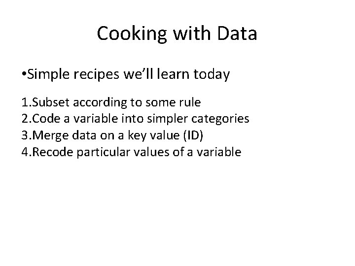
Cooking with Data • Simple recipes we’ll learn today 1. Subset according to some rule 2. Code a variable into simpler categories 3. Merge data on a key value (ID) 4. Recode particular values of a variable

Recipe 1: Subset • object. to. subset[subset instructions] By index By name By logical By expression vector[ c(1, 2, 3) ] data [ 2, 4 ] data [ 3, ] data [ , 2 ] cars[ c(“speed”, ”dist”) ] (1: 3)[ c(TRUE, FALSE, TRUE) ] cars$dist[ cars$speed== 7]

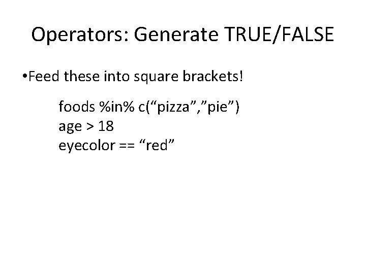
Operators: Generate TRUE/FALSE • Feed these into square brackets! foods %in% c(“pizza”, ”pie”) age > 18 eyecolor == “red”

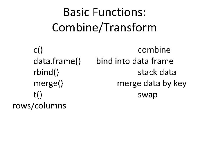
Basic Functions: Combine/Transform c() data. frame() rbind() merge() t() rows/columns combine bind into data frame stack data merge data by key swap

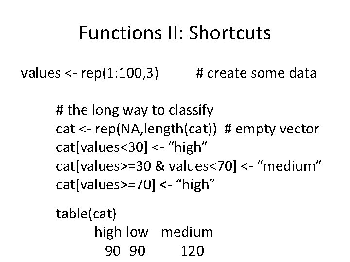
Functions II: Shortcuts values <- rep(1: 100, 3) # create some data # the long way to classify cat <- rep(NA, length(cat)) # empty vector cat[values<30] <- “high” cat[values>=30 & values<70] <- “medium” cat[values>=70] <- “high” table(cat) high low medium 90 90 120

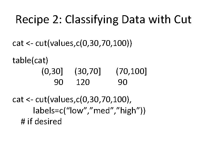
Recipe 2: Classifying Data with Cut cat <- cut(values, c(0, 30, 70, 100)) table(cat) (0, 30] 90 (30, 70] 120 (70, 100] 90 cat <- cut(values, c(0, 30, 70, 100), labels=c(“low”, ”med”, ”high”)) # if desired

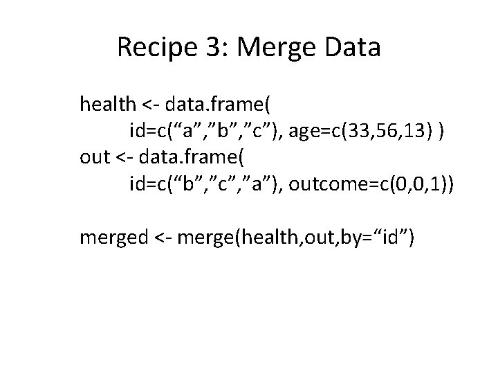
Recipe 3: Merge Data health <- data. frame( id=c(“a”, ”b”, ”c”), age=c(33, 56, 13) ) out <- data. frame( id=c(“b”, ”c”, ”a”), outcome=c(0, 0, 1)) merged <- merge(health, out, by=“id”)

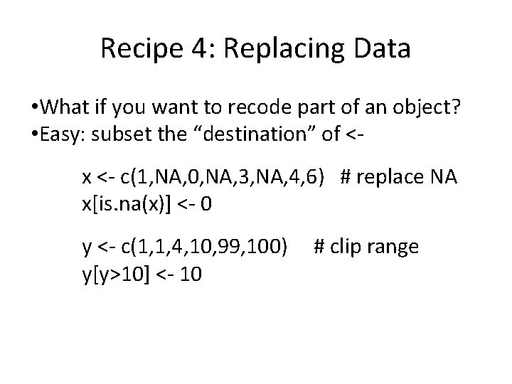
Recipe 4: Replacing Data • What if you want to recode part of an object? • Easy: subset the “destination” of <x <- c(1, NA, 0, NA, 3, NA, 4, 6) # replace NA x[is. na(x)] <- 0 y <- c(1, 1, 4, 10, 99, 100) y[y>10] <- 10 # clip range

Part II: Generalized Linear Models

Why care about Generalized Linear Models (GLMs)? • Almost all Epi models are GLMs –Odds ratios (logistic) –Risk ratios (log-binomial) –“Fancy” models are usually just extensions of GLMs � GWR (geographically weighted regression) adds a “weights matrix” � MCMC (Markov Chain Monte Carlo) solves GLMs with priors

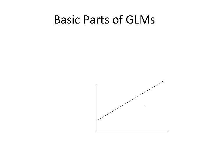
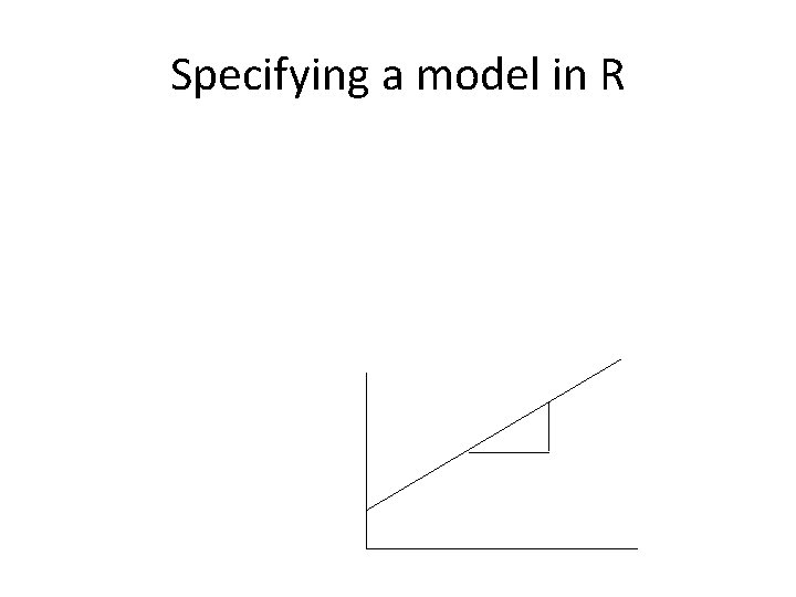
Basic Parts of GLMs

Specifying a model in R

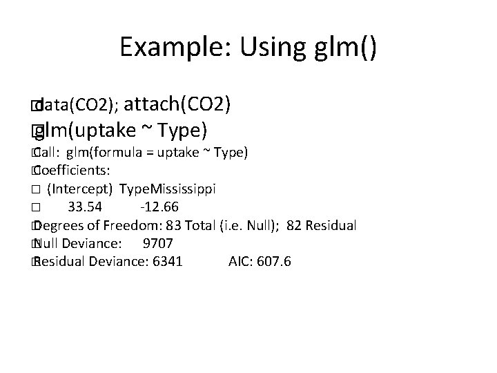
Example: Using glm() � data(CO 2); attach(CO 2) � glm(uptake ~ Type) � Call: glm(formula = uptake ~ Type) � Coefficients: � (Intercept) Type. Mississippi � 33. 54 -12. 66 � Degrees of Freedom: 83 Total (i. e. Null); 82 Residual � Null Deviance: 9707 � Residual Deviance: 6341 AIC: 607. 6

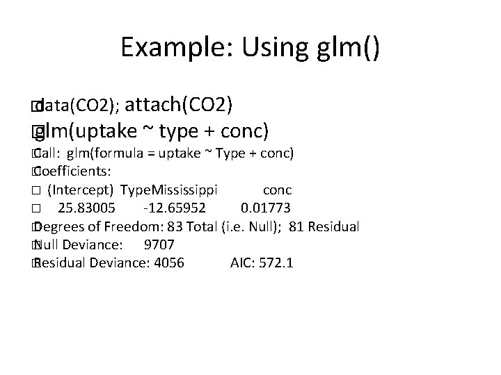
Example: Using glm() � data(CO 2); attach(CO 2) � glm(uptake ~ type + conc) � Call: glm(formula = uptake ~ Type + conc) � Coefficients: � (Intercept) Type. Mississippi conc � 25. 83005 -12. 65952 0. 01773 � Degrees of Freedom: 83 Total (i. e. Null); 81 Residual � Null Deviance: 9707 � Residual Deviance: 4056 AIC: 572. 1

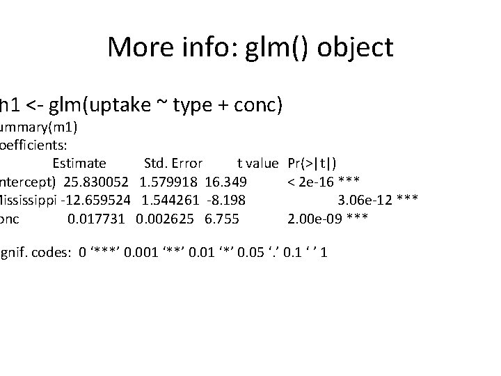
More info: glm() object � m 1 <- glm(uptake ~ type + conc) ummary(m 1) oefficients: Estimate ntercept) 25. 830052 Mississippi -12. 659524 onc 0. 017731 Std. Error t value Pr(>|t|) 1. 579918 16. 349 < 2 e-16 *** 1. 544261 -8. 198 3. 06 e-12 *** 0. 002625 6. 755 2. 00 e-09 *** ignif. codes: 0 ‘***’ 0. 001 ‘**’ 0. 01 ‘*’ 0. 05 ‘. ’ 0. 1 ‘ ’ 1

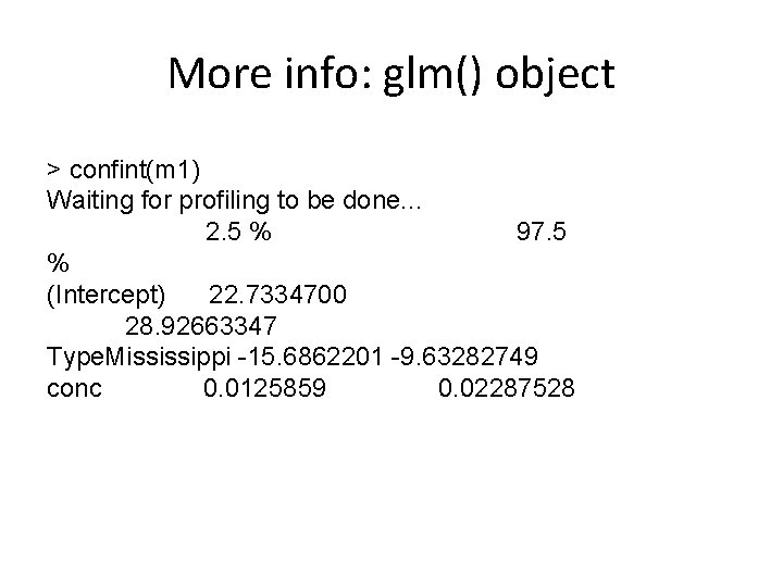
More info: glm() object > confint(m 1) Waiting for profiling to be done. . . 2. 5 % 97. 5 % (Intercept) 22. 7334700 28. 92663347 Type. Mississippi -15. 6862201 -9. 63282749 conc 0. 0125859 0. 02287528

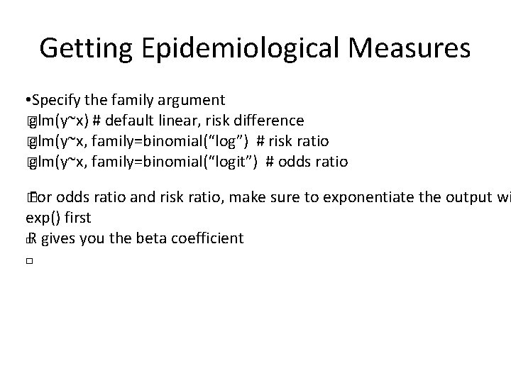
Getting Epidemiological Measures • Specify the family argument � glm(y~x) # default linear, risk difference � glm(y~x, family=binomial(“log”) # risk ratio � glm(y~x, family=binomial(“logit”) # odds ratio � For odds ratio and risk ratio, make sure to exponentiate the output wi exp() first � R gives you the beta coefficient �

Lab: Practice with GLMs • You'll learn more about model-building in courses � What goes in the model (confounders) � Choosing a “best” model • Practice data management � Preparing data for analyses � Formatting/extracting results �