Frank Cowell EC 202 Microeconomics May 2008 Revision

Frank Cowell: EC 202 Microeconomics May 2008 Revision Lecture 2 EC 202: Microeconomic Principles II Frank Cowell

Frank Cowell: EC 202 Microeconomics Objectives of the lecture n n Think more about method for long questions Look at a few Cf. D u u n n 4. 12, 4. 13 5. 1 (7. 8) 9. 6 See how they illustrate method Connect these to past exam questions

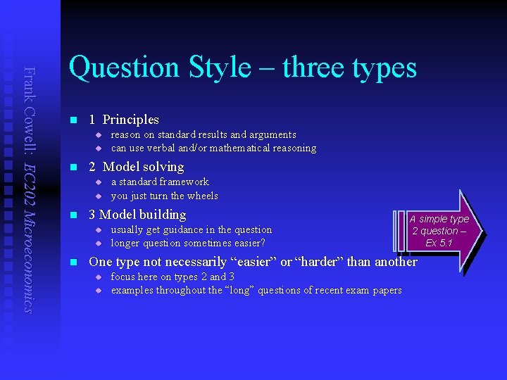
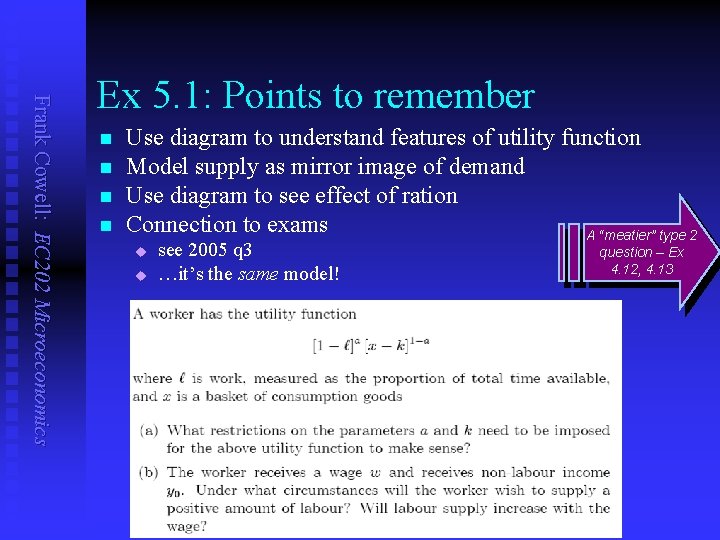
Frank Cowell: EC 202 Microeconomics Question Style – three types n 1 Principles u u n 2 Model solving u u n a standard framework you just turn the wheels 3 Model building u u n reason on standard results and arguments can use verbal and/or mathematical reasoning usually get guidance in the question longer question sometimes easier? A simple type 2 question – Ex 5. 1 One type not necessarily “easier” or “harder” than another u u focus here on types 2 and 3 examples throughout the “long” questions of recent exam papers

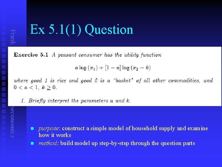
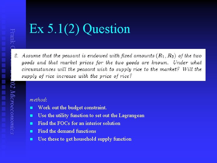
Frank Cowell: EC 202 Microeconomics Ex 5. 1(1) Question n n purpose: construct a simple model of household supply and examine how it works method: build model up step-by-step through the question parts

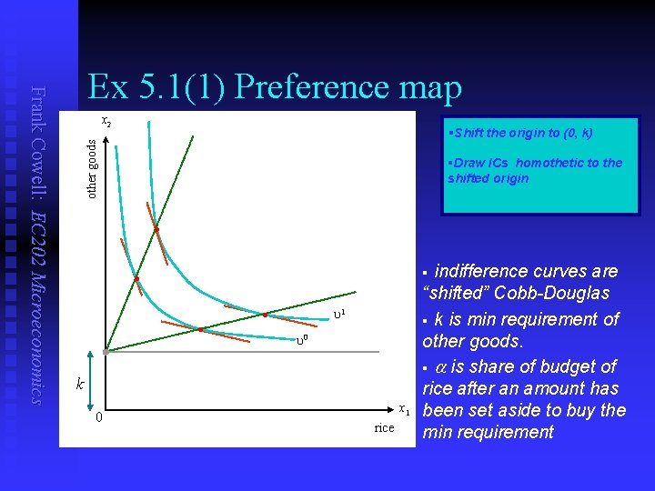
x 2 §Shift the origin to (0, k) other goods Frank Cowell: EC 202 Microeconomics Ex 5. 1(1) Preference map §Draw ICs homothetic to the shifted origin • • • u 1 u 0 k 0 indifference curves are “shifted” Cobb-Douglas § k is min requirement of other goods. § a is share of budget of rice after an amount has been set aside to buy the min requirement § • x 1 rice

Frank Cowell: EC 202 Microeconomics Ex 5. 1(2) Question method: n Work out the budget constraint. n Use the utility function to set out the Lagrangean n Find the FOCs for an interior solution n Find the demand functions n Use these to get household supply function

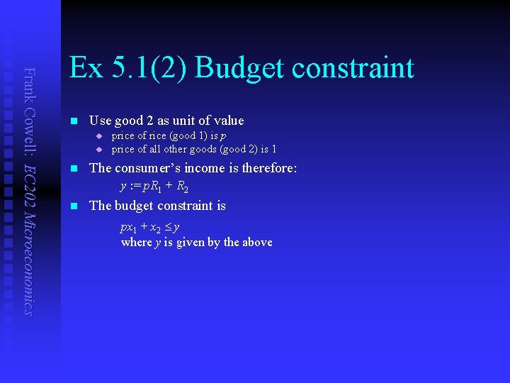
Frank Cowell: EC 202 Microeconomics Ex 5. 1(2) Budget constraint n Use good 2 as unit of value u u n price of rice (good 1) is p price of all other goods (good 2) is 1 The consumer’s income is therefore: y : = p. R 1 + R 2 n The budget constraint is px 1 + x 2 y where y is given by the above

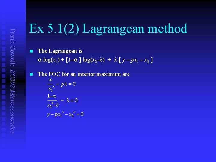
Frank Cowell: EC 202 Microeconomics Ex 5. 1(2) Lagrangean method n The Lagrangean is a log(x 1) + [1–a ] log(x 2–k) + l [ y – px 1 – x 2 ] n The FOC for an interior maximum are a — – pl = 0 x 1 * 1–a —— – l = 0 x 2*–k y – px 1* – x 2* = 0

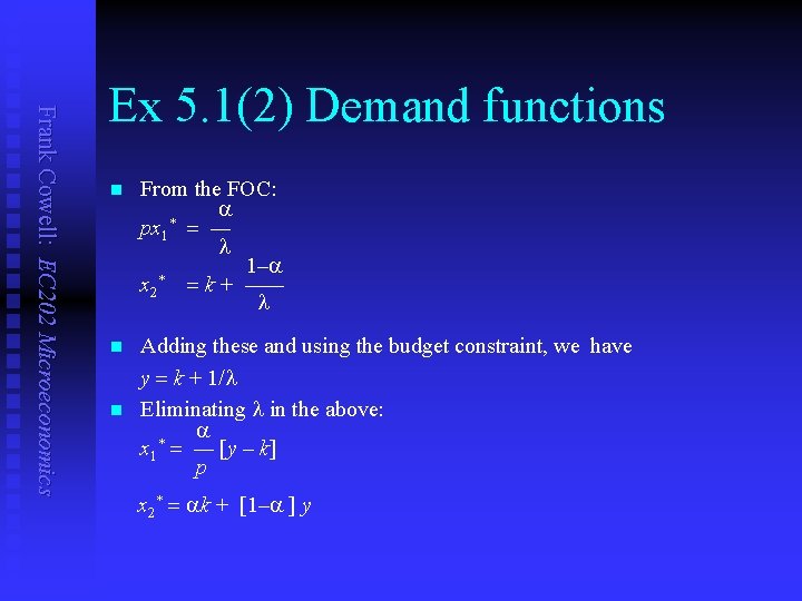
Frank Cowell: EC 202 Microeconomics Ex 5. 1(2) Demand functions n From the FOC: a * px 1 = — l 1–a * x 2 = k + —— l n Adding these and using the budget constraint, we have y = k + 1/l Eliminating l in the above: a * x 1 = — [y – k] p n x 2* = ak + [1–a ] y

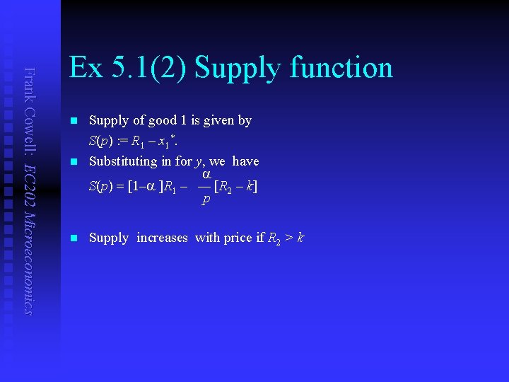
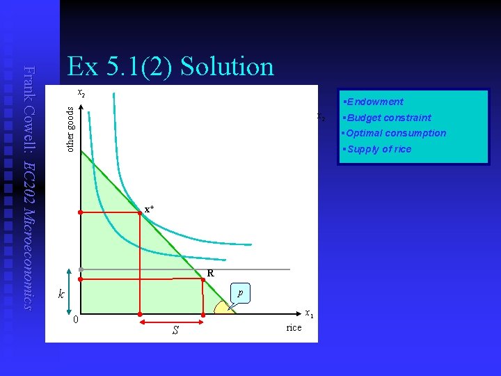
Frank Cowell: EC 202 Microeconomics Ex 5. 1(2) Supply function n Supply of good 1 is given by S(p) : = R 1 – x 1*. Substituting in for y, we have a S(p) = [1–a ]R 1 – — [R 2 – k] p n Supply increases with price if R 2 > k n

x 2 §Endowment other goods Frank Cowell: EC 202 Microeconomics Ex 5. 1(2) Solution x 2 §Optimal consumption §Supply of rice • x* • k 0 §Budget constraint R p x 1 S rice

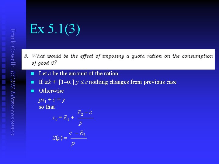
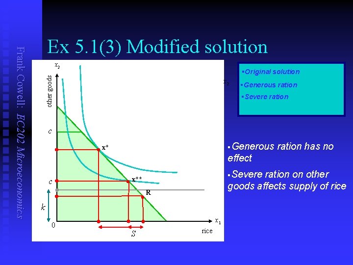
Frank Cowell: EC 202 Microeconomics Ex 5. 1(3) n n n Let c be the amount of the ration If ak + [1–a ] y c nothing changes from previous case Otherwise px 1 + c = y so that R 2 – c x 1 = R 1 + ——— p c – R 2 S(p) = ——— p

x 2 §Original solution other goods Frank Cowell: EC 202 Microeconomics Ex 5. 1(3) Modified solution x 2 §Generous ration §Severe ration c §Generous • x* c effect • §Severe ration on other goods affects supply of rice x** • k 0 ration has no R x 1 S rice

Frank Cowell: EC 202 Microeconomics Ex 5. 1: Points to remember n n Use diagram to understand features of utility function Model supply as mirror image of demand Use diagram to see effect of ration Connection to exams A “meatier” type 2 u u see 2005 q 3 …it’s the same model! question – Ex 4. 12, 4. 13

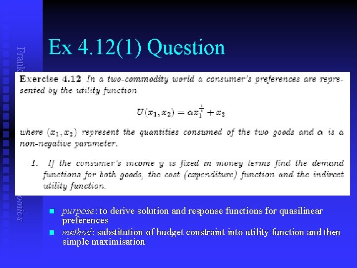
Frank Cowell: EC 202 Microeconomics Ex 4. 12(1) Question n n purpose: to derive solution and response functions for quasilinear preferences method: substitution of budget constraint into utility function and then simple maximisation

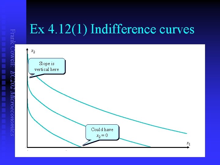
Frank Cowell: EC 202 Microeconomics Ex 4. 12(1) Preliminary n First steps are as follows: n Sketch indifference curves u n Write down budget constraint u n Straightforward – parabolic contours Straightforward – fixed-income case Set out optimisation problem

Frank Cowell: EC 202 Microeconomics Ex 4. 12(1) Indifference curves x 2 Slope is vertical here Could have x 2 = 0 x 1 0 0 1 2

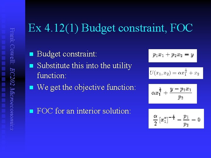
Frank Cowell: EC 202 Microeconomics Ex 4. 12(1) Budget constraint, FOC n Budget constraint: Substitute this into the utility function: We get the objective function: n FOC for an interior solution: n n

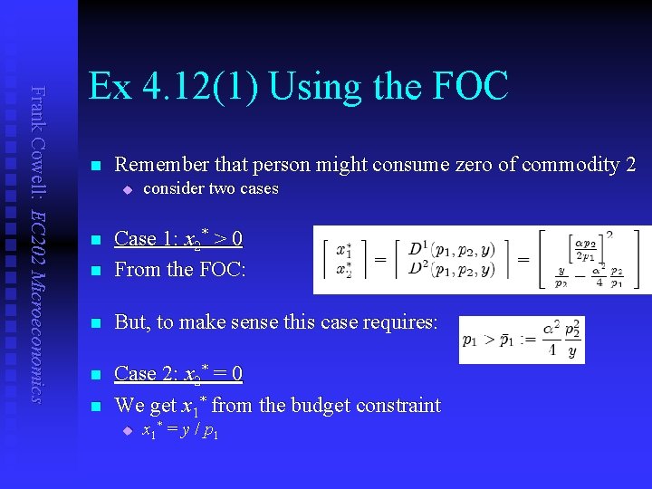
Frank Cowell: EC 202 Microeconomics Ex 4. 12(1) Using the FOC n Remember that person might consume zero of commodity 2 u consider two cases n Case 1: x 2* > 0 From the FOC: n But, to make sense this case requires: n Case 2: x 2* = 0 We get x 1* from the budget constraint n n u x 1* = y / p 1

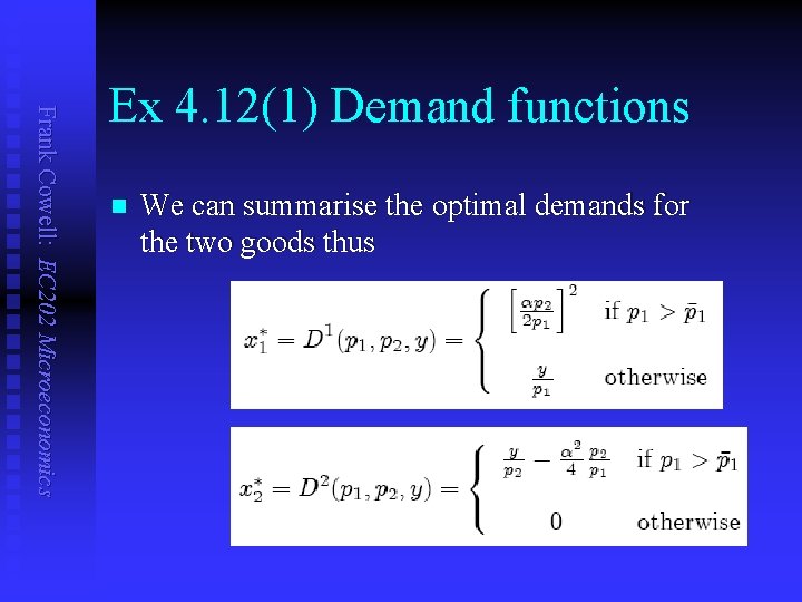
Frank Cowell: EC 202 Microeconomics Ex 4. 12(1) Demand functions n We can summarise the optimal demands for the two goods thus

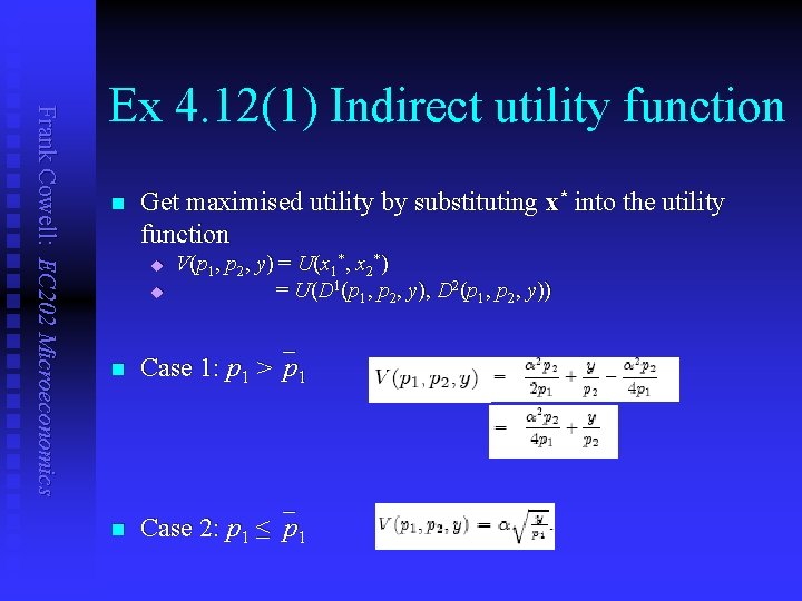
Frank Cowell: EC 202 Microeconomics Ex 4. 12(1) Indirect utility function n Get maximised utility by substituting x* into the utility function u u V(p 1, p 2, y) = U(x 1*, x 2*) = U(D 1(p 1, p 2, y), D 2(p 1, p 2, y)) n Case 1: p 1 >`p 1 n Case 2: p 1 ≤`p 1

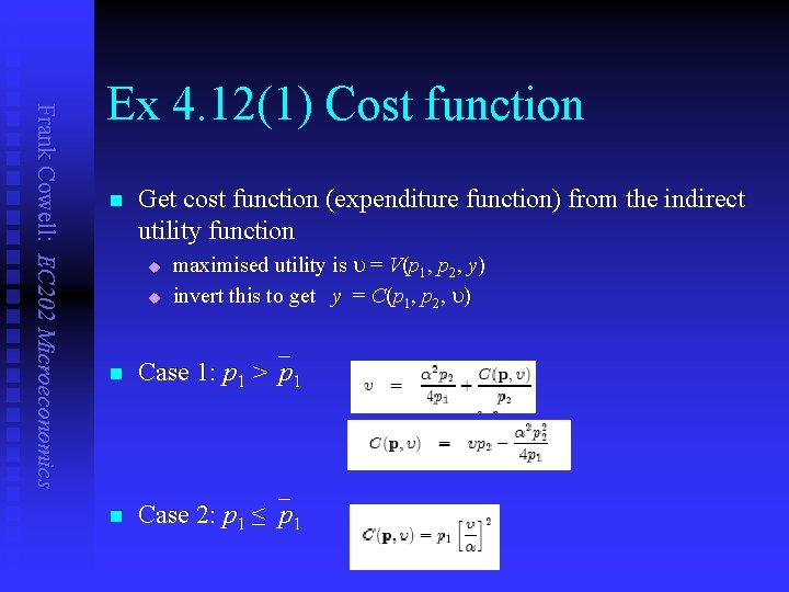
Frank Cowell: EC 202 Microeconomics Ex 4. 12(1) Cost function n Get cost function (expenditure function) from the indirect utility function u u maximised utility is u = V(p 1, p 2, y) invert this to get y = C(p 1 , p 2 , u) n Case 1: p 1 >`p 1 n Case 2: p 1 ≤ `p 1

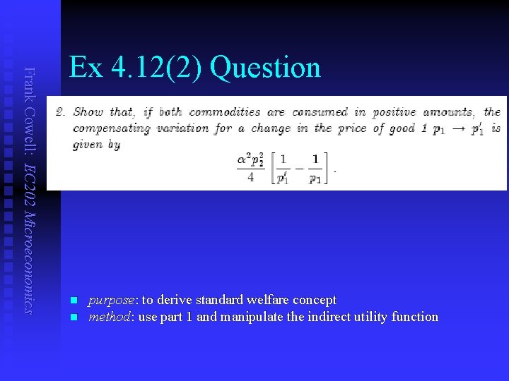
Frank Cowell: EC 202 Microeconomics Ex 4. 12(2) Question n n purpose: to derive standard welfare concept method: use part 1 and manipulate the indirect utility function

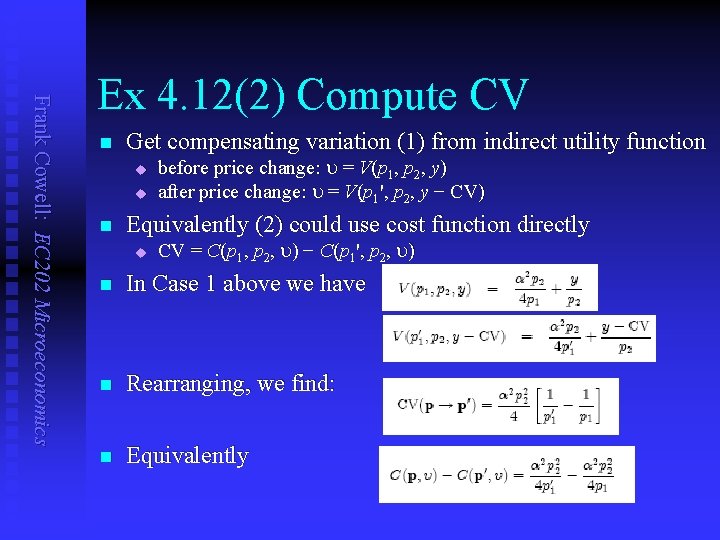
Frank Cowell: EC 202 Microeconomics Ex 4. 12(2) Compute CV n Get compensating variation (1) from indirect utility function u u n before price change: u = V(p 1, p 2, y) after price change: u = V(p 1', p 2, y − CV) Equivalently (2) could use cost function directly u CV = C(p 1, p 2, u) − C(p 1', p 2, u) n In Case 1 above we have n Rearranging, we find: n Equivalently

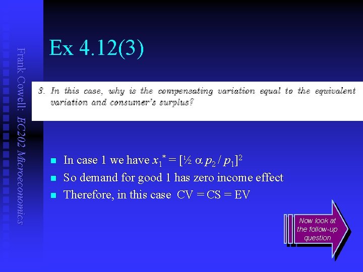
Frank Cowell: EC 202 Microeconomics Ex 4. 12(3) n n n In case 1 we have x 1* = [½ a p 2 / p 1]2 So demand for good 1 has zero income effect Therefore, in this case CV = CS = EV Now look at the follow-up question

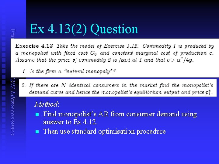
Frank Cowell: EC 202 Microeconomics Ex 4. 13(2) Question Method: n Find monopolist’s AR from consumer demand using answer to Ex 4. 12. n Then use standard optimisation procedure

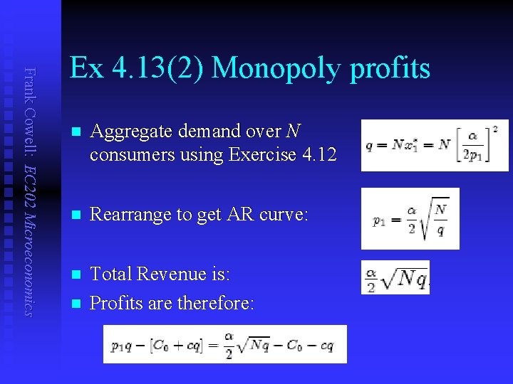
Frank Cowell: EC 202 Microeconomics Ex 4. 13(2) Monopoly profits n Aggregate demand over N consumers using Exercise 4. 12 n Rearrange to get AR curve: n Total Revenue is: Profits are therefore: n

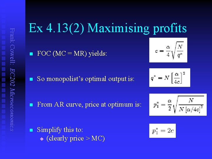
Frank Cowell: EC 202 Microeconomics Ex 4. 13(2) Maximising profits n FOC (MC = MR) yields: n So monopolist’s optimal output is: n From AR curve, price at optimum is: n Simplify this to: u (clearly price > MC)

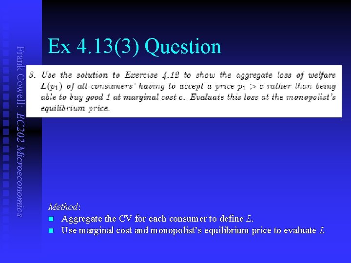
Frank Cowell: EC 202 Microeconomics Ex 4. 13(3) Question Method: n Aggregate the CV for each consumer to define L. n Use marginal cost and monopolist’s equilibrium price to evaluate L

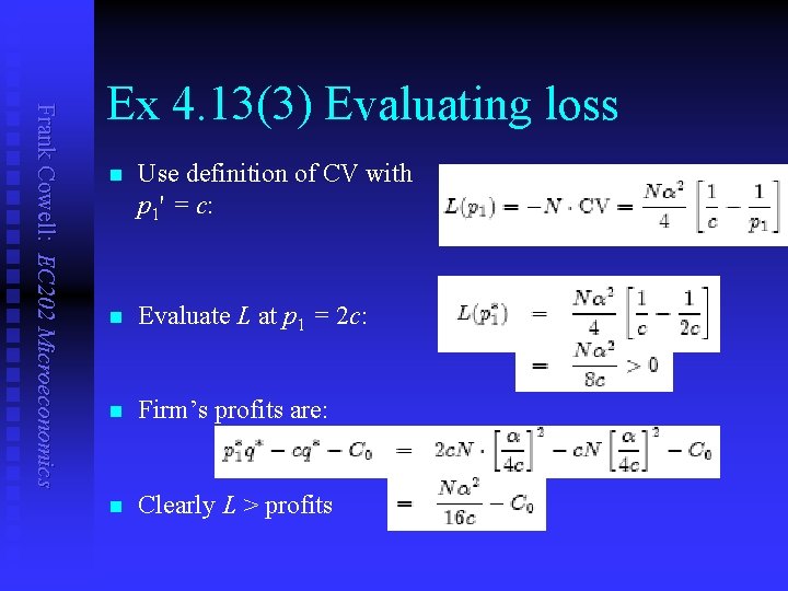
Frank Cowell: EC 202 Microeconomics Ex 4. 13(3) Evaluating loss n Use definition of CV with p 1' = c: n Evaluate L at p 1 = 2 c: n Firm’s profits are: n Clearly L > profits

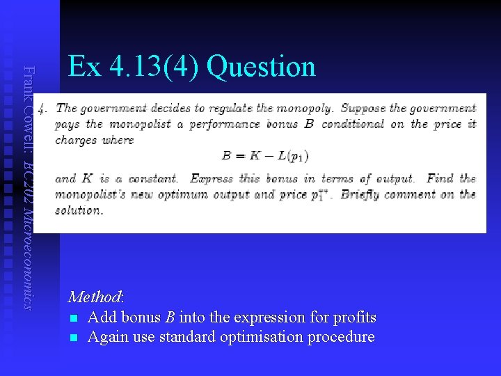
Frank Cowell: EC 202 Microeconomics Ex 4. 13(4) Question Method: n Add bonus B into the expression for profits n Again use standard optimisation procedure

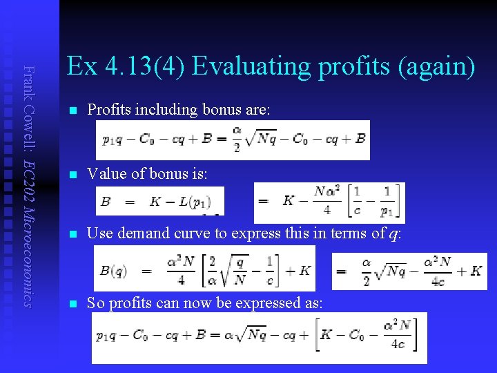
Frank Cowell: EC 202 Microeconomics Ex 4. 13(4) Evaluating profits (again) n Profits including bonus are: n Value of bonus is: n Use demand curve to express this in terms of q: n So profits can now be expressed as:

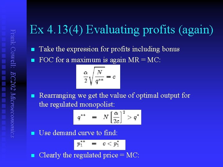
Frank Cowell: EC 202 Microeconomics Ex 4. 13(4) Evaluating profits (again) n n Take the expression for profits including bonus FOC for a maximum is again MR = MC: n Rearranging we get the value of optimal output for the regulated monopolist: n Use demand curve to find: n Clearly the regulated price = MC:

Frank Cowell: EC 202 Microeconomics Ex 4. 12 & 4. 13: Points to note n It’s always a good idea to sketch the indifference curves u u n n A corner solution can sometimes just be handled as two separate cases There’s often more than one way of getting to a solution u n n n in this case the sketch is revealing… …because of the possible corner solution in this case two equivalent derivations of CV Aggregate welfare loss is found from individual CV Unregulated monopoly makes profits smaller than losses to consumer Regulation causes monopoly to behave like competitive firm Now for a type 3 “model building” q

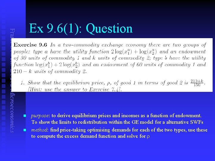
Frank Cowell: EC 202 Microeconomics Ex 9. 6(1): Question n n purpose: to derive equilibrium prices and incomes as a function of endowment. To show the limits to redistribution within the GE model for a alternative SWFs method: find price-taking optimising demands for each of the two types, use these to compute the excess demand function and solve for r

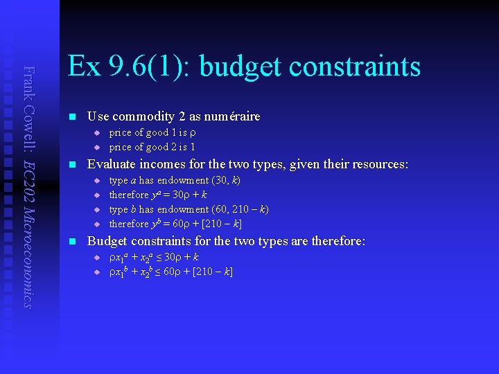
Frank Cowell: EC 202 Microeconomics Ex 9. 6(1): budget constraints n Use commodity 2 as numéraire u u n Evaluate incomes for the two types, given their resources: u u n price of good 1 is r price of good 2 is 1 type a has endowment (30, k) therefore ya = 30 r + k type b has endowment (60, 210 k) therefore yb = 60 r + [210 k] Budget constraints for the two types are therefore: u u rx 1 a + x 2 a ≤ 30 r + k rx 1 b + x 2 b ≤ 60 r + [210 k]

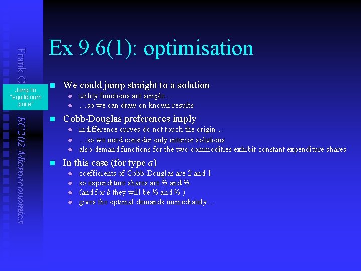
Frank Cowell: EC 202 Microeconomics Jump to “equilibrium price” Ex 9. 6(1): optimisation n We could jump straight to a solution u u n Cobb-Douglas preferences imply u u u n utility functions are simple… …so we can draw on known results indifference curves do not touch the origin… …so we need consider only interior solutions also demand functions for the two commodities exhibit constant expenditure shares In this case (for type a) u u coefficients of Cobb-Douglas are 2 and 1 so expenditure shares are ⅔ and ⅓ (and for b they will be ⅓ and ⅔ ) gives the optimal demands immediately…

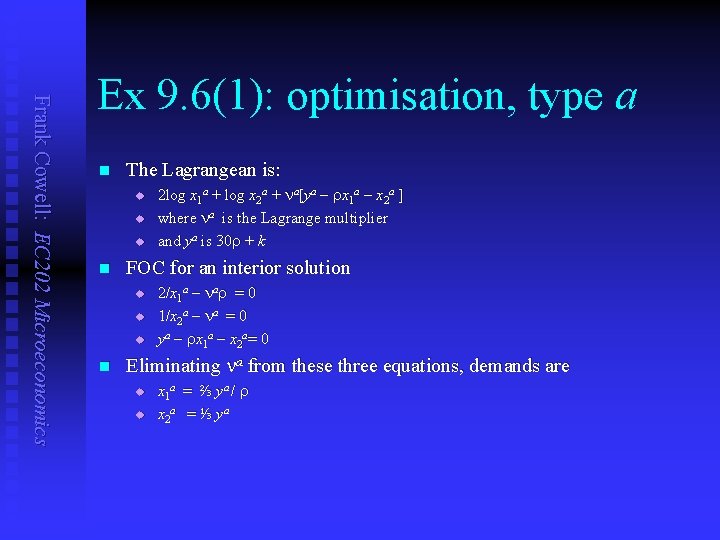
Frank Cowell: EC 202 Microeconomics Ex 9. 6(1): optimisation, type a n The Lagrangean is: u u u n FOC for an interior solution u u u n 2 log x 1 a + log x 2 a + na [ya rx 1 a x 2 a ] where na is the Lagrange multiplier and ya is 30 r + k 2/x 1 a nar = 0 1/x 2 a na = 0 ya rx 1 a x 2 a = 0 Eliminating na from these three equations, demands are u u x 1 a = ⅔ ya / r x 2 a = ⅓ ya

Frank Cowell: EC 202 Microeconomics Ex 9. 6(1): optimisation, type b n The Lagrangean is: u u u n FOC for an interior solution u u u n log x 1 b + 2 log x 2 b + nb [yb rx 1 b x 2 b ] where nb is the Lagrange multiplier and yb is 60 r + 210 k 1/x 1 b nbr = 0 2/x 2 b nb = 0 yb rx 1 b x 2 b= 0 Eliminating nb from these three equations, demands are u x 1 b = ⅓ yb / r u x 2 b = ⅔yb

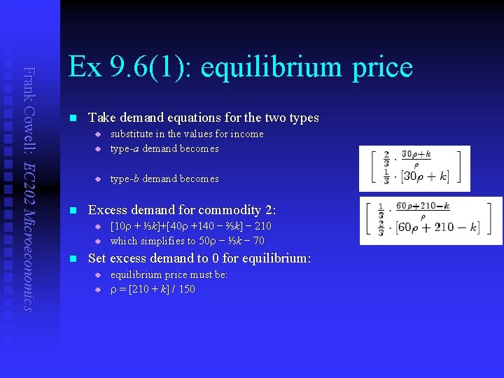
Frank Cowell: EC 202 Microeconomics Ex 9. 6(1): equilibrium price n Take demand equations for the two types u substitute in the values for income type-a demand becomes u type-b demand becomes u n Excess demand for commodity 2: u u n [10 r + ⅓k]+[40 r +140 − ⅔k] − 210 which simplifies to 50 r − ⅓k − 70 Set excess demand to 0 for equilibrium: u u equilibrium price must be: r = [210 + k] / 150

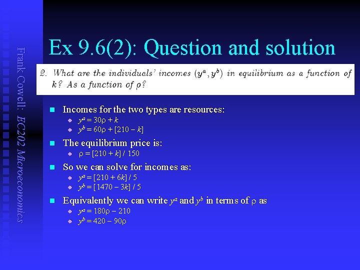
Frank Cowell: EC 202 Microeconomics Ex 9. 6(2): Question and solution n Incomes for the two types are resources: u u n The equilibrium price is: u n r = [210 + k] / 150 So we can solve for incomes as: u u n ya = 30 r + k yb = 60 r + [210 k] ya = [210 + 6 k] / 5 yb = [1470 3 k] / 5 Equivalently we can write ya and yb in terms of r as u u ya = 180 r 210 yb = 420 90 r

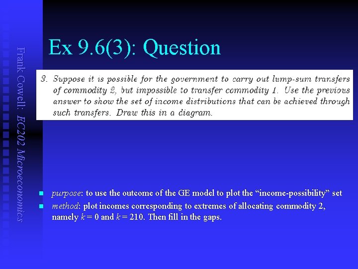
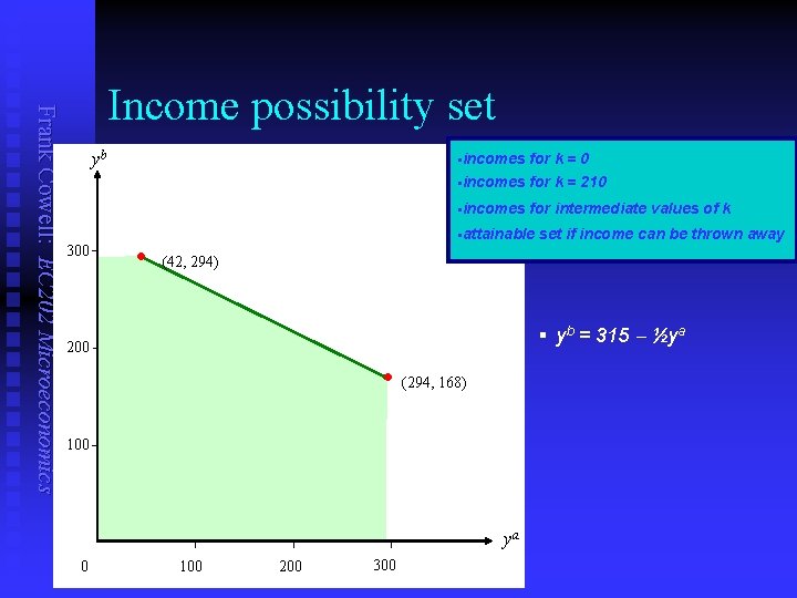
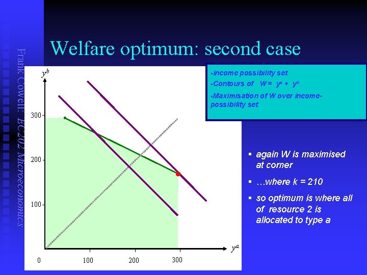
Frank Cowell: EC 202 Microeconomics Ex 9. 6(3): Question n n purpose: to use the outcome of the GE model to plot the “income-possibility” set method: plot incomes corresponding to extremes of allocating commodity 2, namely k = 0 and k = 210. Then fill in the gaps.

Frank Cowell: EC 202 Microeconomics Income possibility set yb 300 • §incomes for k = 0 §incomes for k = 210 §incomes for intermediate values of k §attainable (42, 294) § yb = 315 ½ya 200 • (294, 168) 100 ya 0 set if income can be thrown away 100 200 300

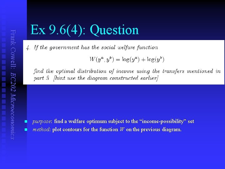
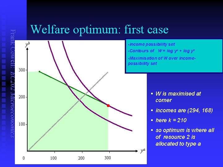
Frank Cowell: EC 202 Microeconomics Ex 9. 6(4): Question n n purpose: find a welfare optimum subject to the “income-possibility” set method: plot contours for the function W on the previous diagram.

Frank Cowell: EC 202 Microeconomics Welfare optimum: first case yb §income possibility set §Contours of W = log ya + log yb §Maximisation of W over income- possibility set 300 § W is maximised at 200 corner • § incomes are (294, 168) § here k = 210 100 § so optimum is where all of resource 2 is allocated to type a ya 0 100 200 300

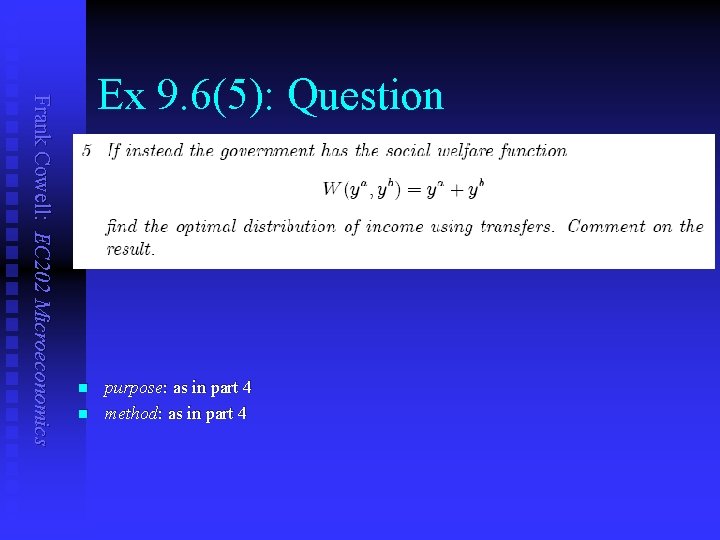
Frank Cowell: EC 202 Microeconomics Ex 9. 6(5): Question n n purpose: as in part 4 method: as in part 4

Frank Cowell: EC 202 Microeconomics Welfare optimum: second case yb §income possibility set §Contours of W = ya + yb §Maximisation of W over income- possibility set 300 § again W is maximised 200 at corner • § …where k = 210 § so optimum is where all 100 of resource 2 is allocated to type a ya 0 100 200 300

Frank Cowell: EC 202 Microeconomics Ex 9. 6: Points to note n n Applying GE methods gives the feasible set Limits to redistribution u u n n Must take account of corners Get the same W-maximising solution u u n where society is averse to inequality where society is indifferent to inequality Link to exam u u u n natural bounds on k asymmetric attainable set very similar to 2007 q 5. but also check out 2005 q 4… …same model, but you are asked to different tricks with it More practice with GE – see Cf. D 7. 8