Intermediate Microeconomics and Its Application 10 th Edition

Intermediate Microeconomics and Its Application 10 th Edition by Walter Nicholson, Amherst College Christopher Snyder, Dartmouth College Power. Point Slide Presentation by Mark Karscig Central Missouri State University © 2006 Thomson Learning/South-Western

Chapter 1 Economic Models © 2004 Thomson Learning/South-Western

Economics n How societies allocate scarce resources among alternative uses—three questions: n What to produce n How much to produce n Who gets the physical and monetary proceeds 3

MICROECONOMICS 4 n How individuals and firms make economic choices among scarce resources n How these choices create markets

Economic Models Simple theoretical descriptions--capture essentials of how economies work n n Real economies too complex to describe in useful detail Models are unrealistic, but useful n 5 Maps unrealistic--do not show every house, parking lot, etc. Despite lack of “realism, ” maps show overall picture; help us get where we want to go; form mental image

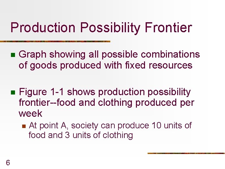
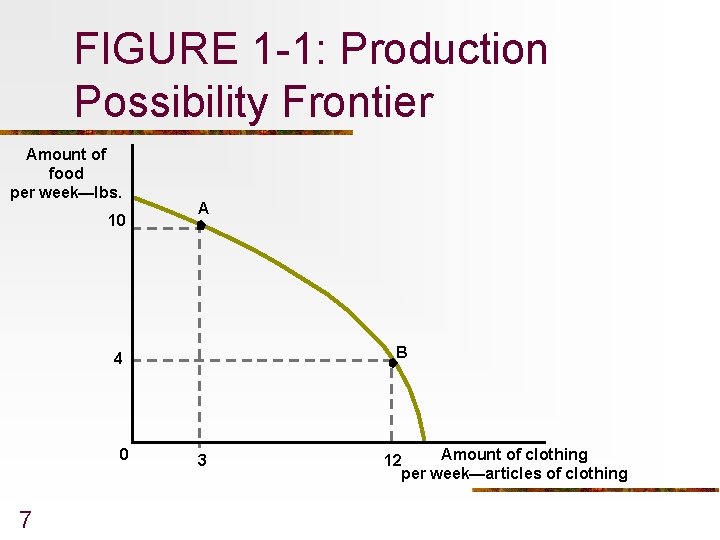
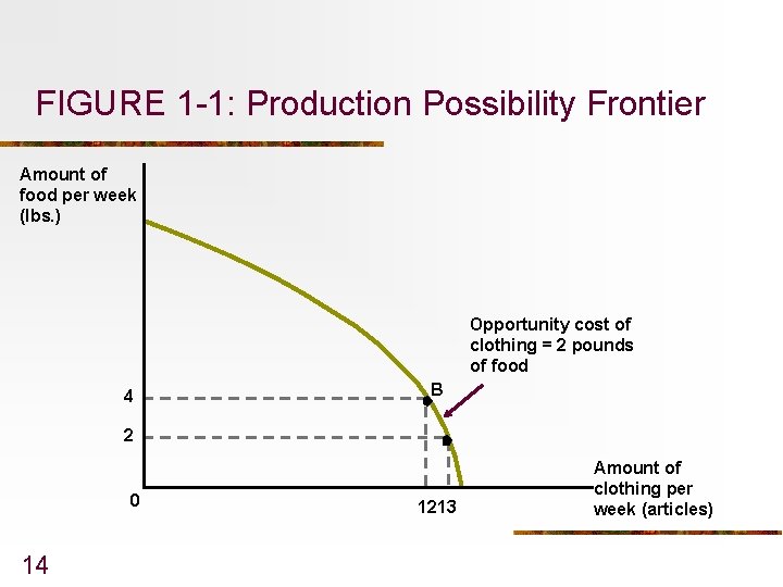
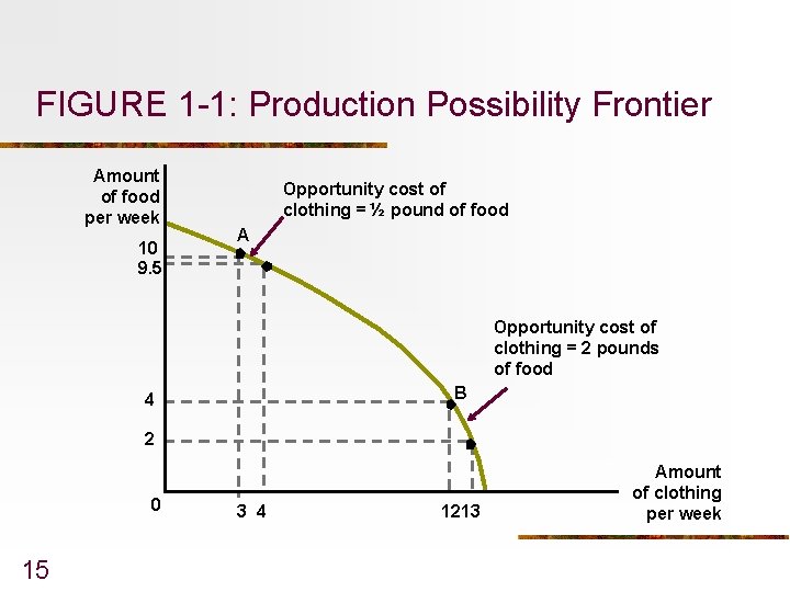
Production Possibility Frontier n Graph showing all possible combinations of goods produced with fixed resources n Figure 1 -1 shows production possibility frontier--food and clothing produced per week n 6 At point A, society can produce 10 units of food and 3 units of clothing

FIGURE 1 -1: Production Possibility Frontier Amount of food per week—lbs. 10 A B 4 0 7 3 Amount of clothing 12 per week—articles of clothing

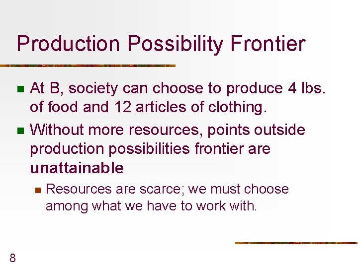
Production Possibility Frontier n n At B, society can choose to produce 4 lbs. of food and 12 articles of clothing. Without more resources, points outside production possibilities frontier are unattainable n 8 Resources are scarce; we must choose among what we have to work with.

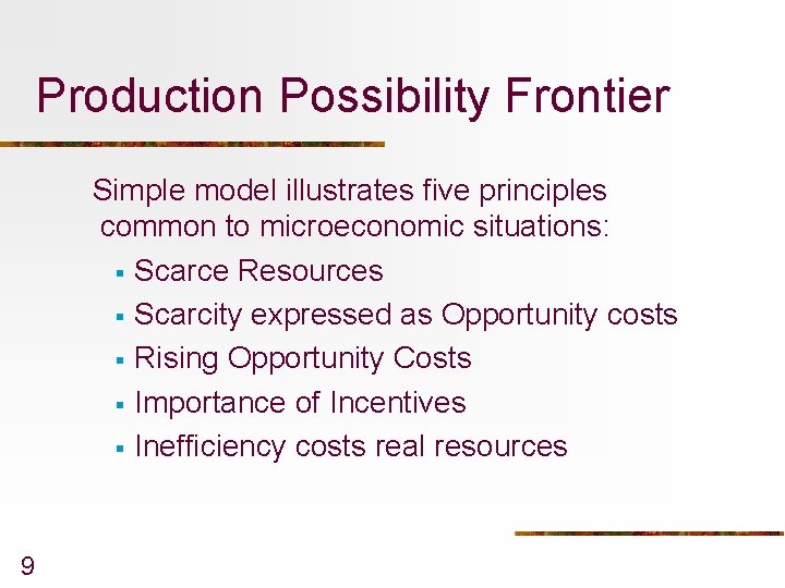
Production Possibility Frontier Simple model illustrates five principles common to microeconomic situations: § Scarce Resources § Scarcity expressed as Opportunity costs § Rising Opportunity Costs § Importance of Incentives § Inefficiency costs real resources 9

Scarcity And Opportunity Costs Opportunity cost: n Cost of a good as measured by goods or services that could have been produced using those scarce resources 10

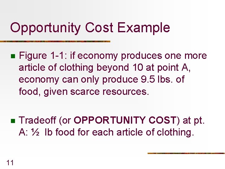
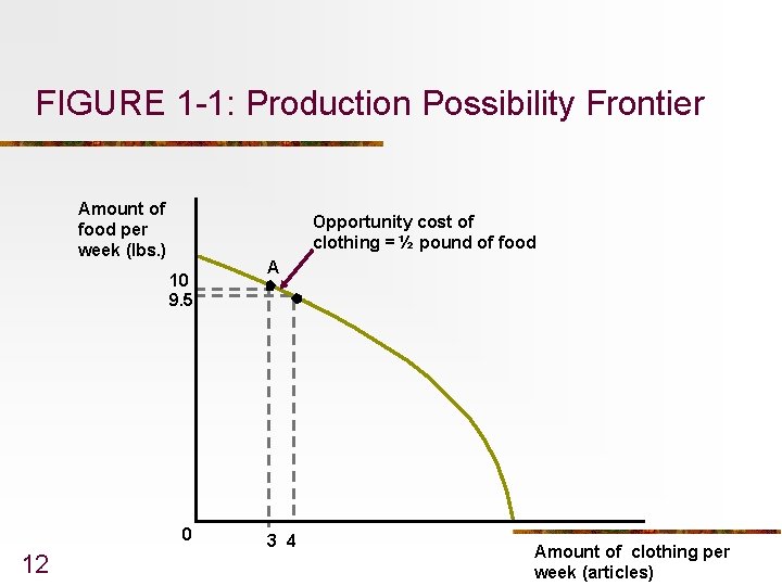
Opportunity Cost Example n Figure 1 -1: if economy produces one more article of clothing beyond 10 at point A, economy can only produce 9. 5 lbs. of food, given scarce resources. n Tradeoff (or OPPORTUNITY COST) at pt. A: ½ lb food for each article of clothing. 11

FIGURE 1 -1: Production Possibility Frontier Amount of food per week (lbs. ) Opportunity cost of clothing = ½ pound of food 10 9. 5 0 12 A 3 4 Amount of clothing per week (articles)

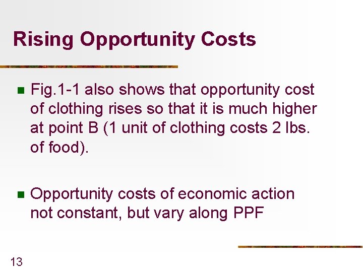
Rising Opportunity Costs n Fig. 1 -1 also shows that opportunity cost of clothing rises so that it is much higher at point B (1 unit of clothing costs 2 lbs. of food). n Opportunity costs of economic action not constant, but vary along PPF 13

FIGURE 1 -1: Production Possibility Frontier Amount of food per week (lbs. ) Opportunity cost of clothing = 2 pounds of food 4 B 2 0 14 1213 Amount of clothing per week (articles)

FIGURE 1 -1: Production Possibility Frontier Amount of food per week 10 9. 5 Opportunity cost of clothing = ½ pound of food A Opportunity cost of clothing = 2 pounds of food B 4 2 0 15 3 4 1213 Amount of clothing per week

Uses of Microeconomics n Uses of microeconomic analysis vary. One useful way to categorize: by user type: n n n 16 Individuals making decisions regarding jobs, purchases, and finances; Businesses making decisions regarding product demand or production costs, or Governments making policy decisions about economic effects of various proposed or existing laws and regulations.

Basic Supply-Demand Model n n 17 Model describes how sellers’ and buyers’ behavior determines good’s price Economists hold that market behavior generally explained by relationship between buyers’ preferences for a good (demand) and firms’ costs involved in bringing that good to market (supply).

Adam Smith--The Invisible Hand n n n 18 Adam Smith (1723 -1790) saw prices as force that directed resources into activities where resources were most valuable. Prices told both consumers and firms the “worth” of goods. Smith’s somewhat incomplete explanation for prices: determined by the costs to produce the goods.

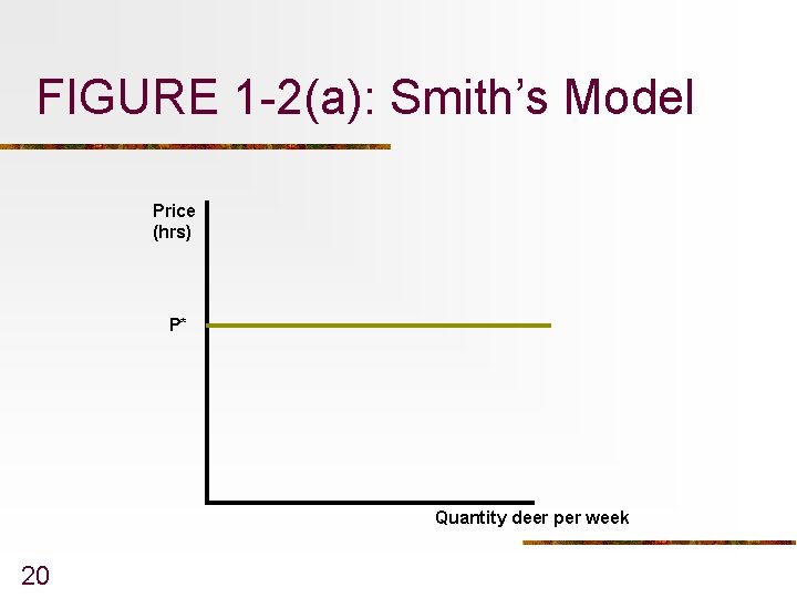
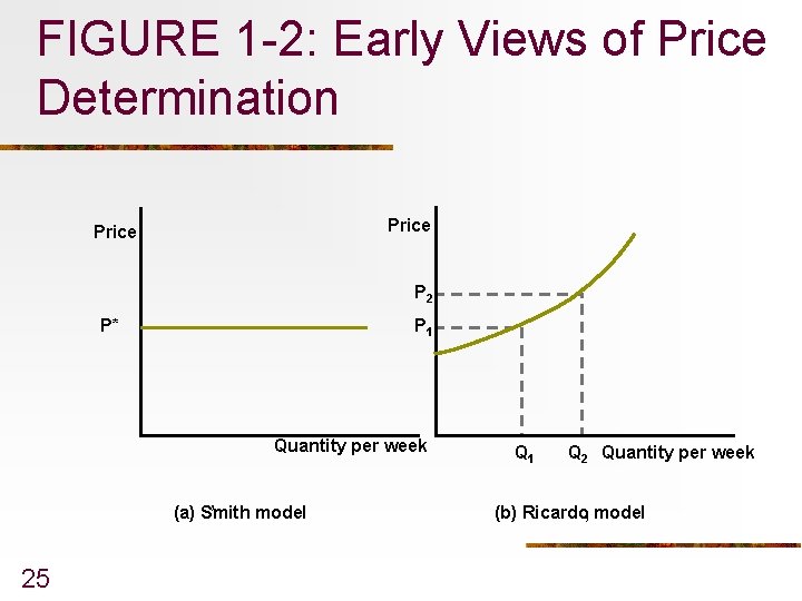
Adam Smith--the Invisible Hand n 19 In 18 th century, labor was primary resource. Thus Smith embraced labor-based theory of prices: n If catching a deer took twice as long as catching a beaver, one deer should trade for two beaver (the relative price of a deer is two beavers). n Figure 1 -2(a), horizontal line at P* shows that any number of deer can be produced without affecting relative cost

FIGURE 1 -2(a): Smith’s Model Price (hrs) P* Quantity deer per week 20

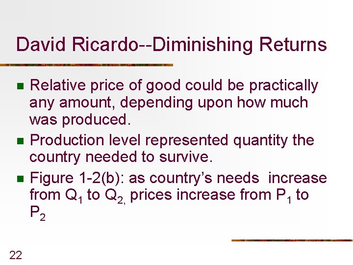
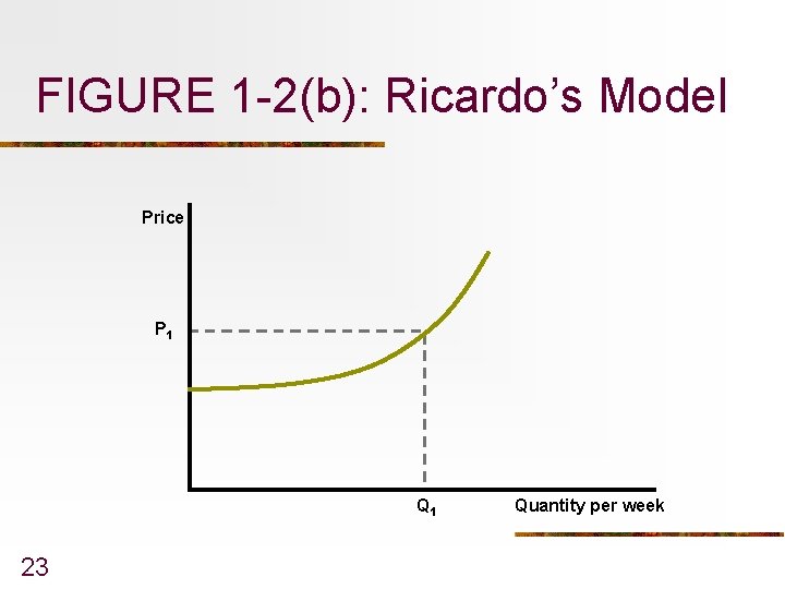
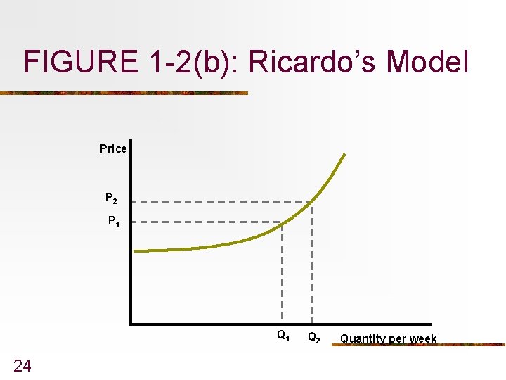
David Ricardo--Diminishing Returns n David Ricardo (1772 -1823) believed that labor and other costs would rise with production level n n 21 As new, less fertile, land was cultivated, farming would require more labor for same yield Increasing cost argument: now referred to as the Law of Diminishing Returns

David Ricardo--Diminishing Returns n n n 22 Relative price of good could be practically any amount, depending upon how much was produced. Production level represented quantity the country needed to survive. Figure 1 -2(b): as country’s needs increase from Q 1 to Q 2, prices increase from P 1 to P 2

FIGURE 1 -2(b): Ricardo’s Model Price P 1 Q 1 23 Quantity per week

FIGURE 1 -2(b): Ricardo’s Model Price P 2 P 1 Q 1 24 Q 2 Quantity per week

FIGURE 1 -2: Early Views of Price Determination Price P 2 P* P 1 Quantity per week (a) Smith ’ model 25 Q 1 Q 2 Quantity per week (b) Ricardo model ’

Marshall’s Model of Supply and Demand n n 26 Ricardo’s model could not explain fall in relative good prices during nineteenth century (industrialization), so economists needed a more general model. Economists argued that people’s willingness to pay for a good will decline as they have more of that good—the beginnings of thinking at the margin.

Marshall, Supply and Demand, and the Margin n 27 People willing to consume more of good only if price drops. Focus of model: on value of last, or marginal, unit purchased Alfred Marshall (1842 -1924) showed how forces of demand supply simultaneously determined price.

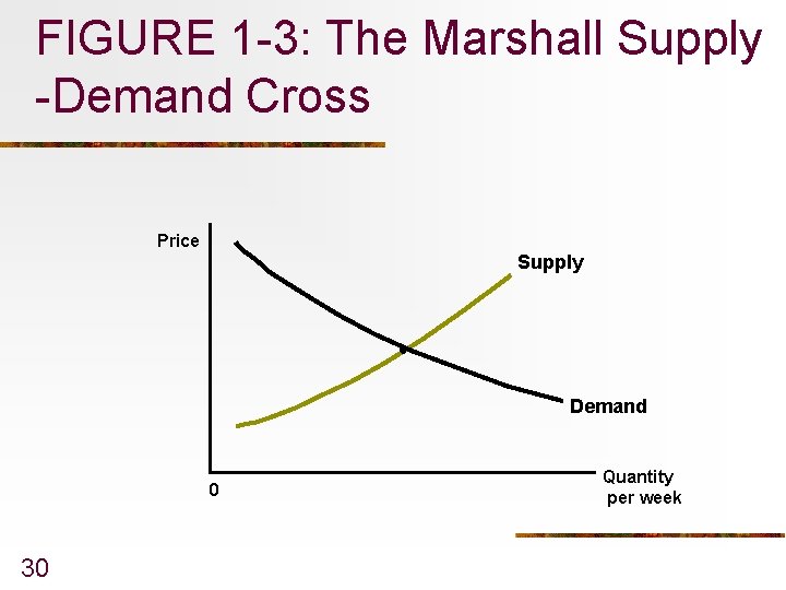
Marshall, Supply and Demand, and the Margin n Figure 1 -3: amount of good purchased period shown on the horizontal axis; price of good appears on vertical axis. n Demand curve shows amount of good people want to buy at each price. Negative slope reflects marginalist principle. 28

Marshall, Supply and Demand, and the Margin n n 29 Upward-sloping supply curve reflects increasing cost of making one more unit of a good as total amount produced increases. Supply reflects increasing marginal costs and demand reflects decreasing marginal utility.

FIGURE 1 -3: The Marshall Supply -Demand Cross Price Supply Demand 0 30 Quantity per week

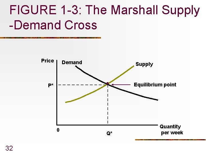
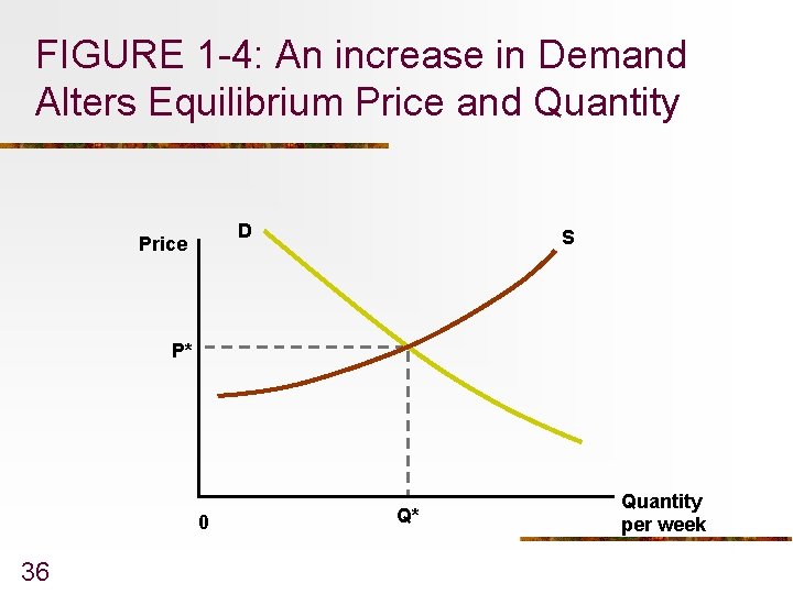
Market Equilibrium n n 31 Figure 1 -3: demand supply curves intersect at the market equilibrium point P*, Q* P* is equilibrium price: price at which the quantity demanded by a good’s buyers precisely equals quantity of that good supplied by sellers

FIGURE 1 -3: The Marshall Supply -Demand Cross Price Demand . P* 0 32 Q* Supply Equilibrium point Quantity per week

Market Equilibrium n n 33 Both buyers and sellers are satisfied at this price--no incentive for either to alter their behavior unless something else changes Marshall compared roles of supply and demand in establishing market equilibrium to two scissor blades working together in order to make a cut

Non-equilibrium Outcomes n n 34 If an event causes the price to be set above P*, demanders would wish to buy less than Q, * while suppliers would produce more than Q*. If something causes the price to be set below P*, demanders would wish to buy more than Q* while suppliers would produce less than Q*.

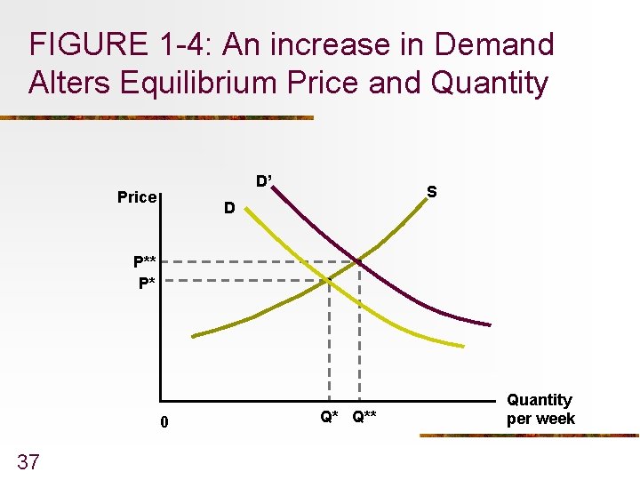
Change in Market Equilibrium: Increased Demand n n 35 Figure 1 -4 people’s demand for good increases, as represented by shift of demand curve from D to D’ New equilibrium established where equilibrium price increases to P**

FIGURE 1 -4: An increase in Demand Alters Equilibrium Price and Quantity D Price S P* 0 36 Q* Quantity per week

FIGURE 1 -4: An increase in Demand Alters Equilibrium Price and Quantity D’ Price S D P** P* 0 37 Q* Q** Quantity per week

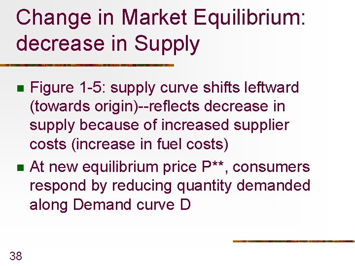
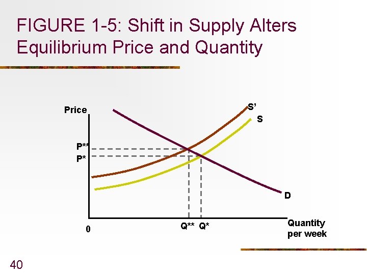
Change in Market Equilibrium: decrease in Supply n n 38 Figure 1 -5: supply curve shifts leftward (towards origin)--reflects decrease in supply because of increased supplier costs (increase in fuel costs) At new equilibrium price P**, consumers respond by reducing quantity demanded along Demand curve D

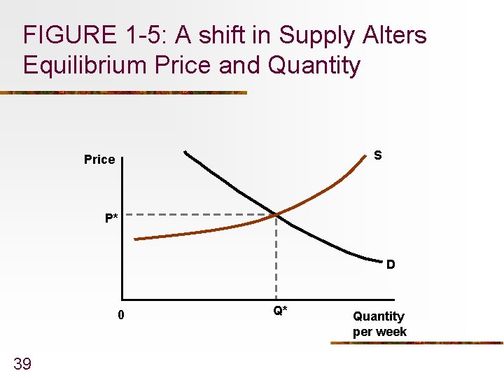
FIGURE 1 -5: A shift in Supply Alters Equilibrium Price and Quantity S Price P* D 0 39 Q* Quantity per week

FIGURE 1 -5: Shift in Supply Alters Equilibrium Price and Quantity S’ Price S P** P* D 0 40 Q** Q* Quantity per week

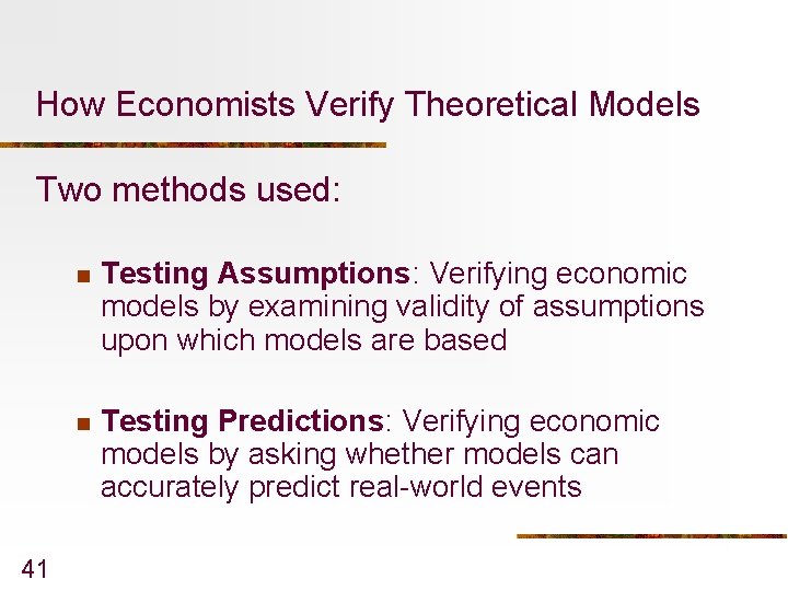
How Economists Verify Theoretical Models Two methods used: 41 n Testing Assumptions: Verifying economic models by examining validity of assumptions upon which models are based n Testing Predictions: Verifying economic models by asking whether models can accurately predict real-world events

Testing Assumptions One approach: determine whether underlying assumptions are reasonable n n Empirical evidence n 42 Obvious problem: people differ in opinion of what is reasonable Results have problems similar to those found in opinion polls: interpretation

Testing Predictions n n Economists such as Milton Friedman argue that all theories require unrealistic assumptions. Theory is only useful if it can be used to predict real-world events. n 43 Even if firms state they don’t maximize profits, if their behavior can be predicted by using theory, it is useful.

Models of Many Markets n n 44 Marshall's supply and demand model is partial equilibrium model: Economic model of a single market To show effects of change in one market on others requires a general equilibrium model: An economic model of complete system of markets

Positive-Normative Distinction n Distinguish between theories that seek to explain the world as it is and theories that postulate the way the world should be n n 45 To many economists, the correct role for theory is to explain the way the world is (positive) rather than the way it should be (normative). Text takes approach based on positive economics.