Prerequisites Almost essential Risk Frank Cowell Microeconomics June

Prerequisites Almost essential Risk Frank Cowell: Microeconomics June 2004 Moral Hazard MICROECONOMICS Principles and Analysis Frank Cowell

The moral hazard problem Frank Cowell: Microeconomics n n n u Jump to “Adverse selection” Jump to “Signalling” A key aspect of hidden information Information relates to actions. Hidden action by one party affects probability of favourable/unfavourable outcomes. u u n n Hidden information about personal characteristics is dealt with. . . under “adverse selection. ”. . . under “signalling. ” However similar issues arise in setting up the economic problem. Set-up based on model of trade under uncertainty.

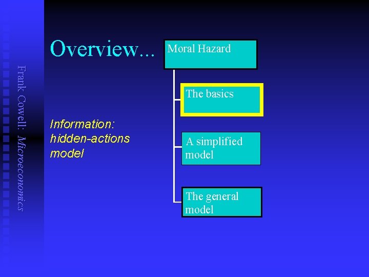
Overview. . . Moral Hazard Frank Cowell: Microeconomics The basics Information: hidden-actions model A simplified model The general model

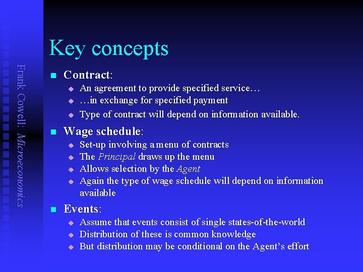
Key concepts Frank Cowell: Microeconomics n Contract: u u u n Wage schedule: u u n An agreement to provide specified service… …in exchange for specified payment Type of contract will depend on information available. Set-up involving a menu of contracts The Principal draws up the menu Allows selection by the Agent Again the type of wage schedule will depend on information available Events: u u u Assume that events consist of single states-of-the-world Distribution of these is common knowledge But distribution may be conditional on the Agent’s effort

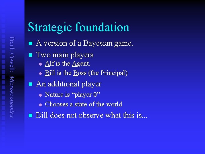
Strategic foundation Frank Cowell: Microeconomics n n A version of a Bayesian game. Two main players u u n An additional player u u n Alf is the Agent. Bill is the Boss (the Principal) Nature is “player 0” Chooses a state of the world Bill does not observe what this is. . .

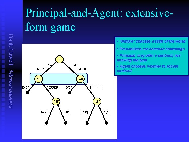
Principal-and-Agent: extensiveform game Frank Cowell: Microeconomics § "Nature" chooses a state of the world § Probabilities are common knowledge 0 p [RED] 1 -p Bill [NO] § Principal may offer a contract, not knowing the type § Agent chooses whether to accept contract [BLUE] Bill [OFFER] [NO] Alf [low] Alf [high] [low] [high]

Extension of trading model Frank Cowell: Microeconomics n Start with trading model under uncertainty u u u n Assume: u u u n A single physical good… …so consumption in each state-of-the world is a distinct “contingent good”. Two traders Alf, Bill CE in Edgeworth box determined as usual: u u n There are two states-of-the world So exactly two possible events Probabilities of the two events are common knowledge Draw a common tangent through the endowment point. Gives equilibrium prices and allocation But what happens in noncompetitive world? u Suppose Bill can completely exploit Alf

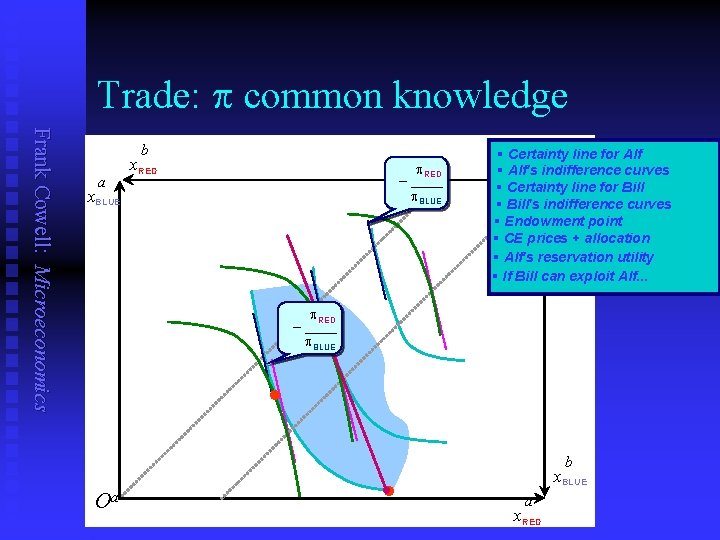
Trade: p common knowledge Frank Cowell: Microeconomics b a x. RED p. RED – ____ p. BLUE x. BLUE § Certainty line for Alf b § Alf's indifference curves O § Certainty line for Bill § Bill's indifference curves § Endowment point § CE prices + allocation § Alf's reservation utility § If Bill can exploit Alf. . . p. RED – ____ p. BLUE • • Oa • b x. BLUE a x. RED

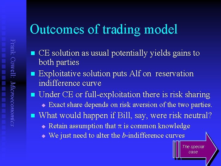
Outcomes of trading model Frank Cowell: Microeconomics n n n CE solution as usual potentially yields gains to both parties Exploitative solution puts Alf on reservation indifference curve Under CE or full-exploitation there is risk sharing u n Exact share depends on risk aversion of the two parties. What would happen if Bill, say, were risk neutral? u u Retain assumption that p is common knowledge We just need to alter the b-indifference curves The special case

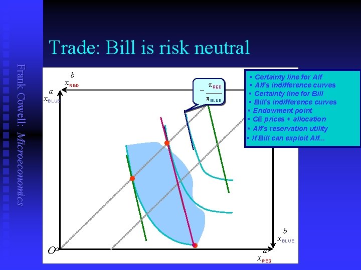
Trade: Bill is risk neutral Frank Cowell: Microeconomics b a x. RED p. RED – ____ p. BLUE x. BLUE • § Certainty line for Alf b § Alf's indifference curves O § Certainty line for Bill § Bill's indifference curves § Endowment point § CE prices + allocation § Alf's reservation utility § If Bill can exploit Alf. . . • Oa • b x. BLUE a x. RED

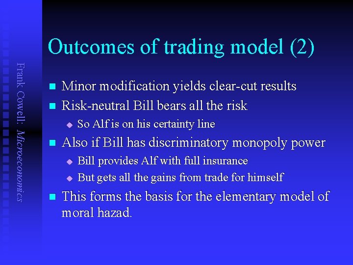
Outcomes of trading model (2) Frank Cowell: Microeconomics n n Minor modification yields clear-cut results Risk-neutral Bill bears all the risk u n Also if Bill has discriminatory monopoly power u u n So Alf is on his certainty line Bill provides Alf with full insurance But gets all the gains from trade for himself This forms the basis for the elementary model of moral hazad.

Overview. . . Moral Hazard Frank Cowell: Microeconomics The basics Lessons from the 2 x 2 case A simplified model The general model

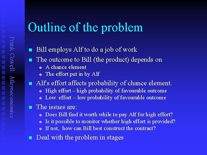
Outline of the problem Frank Cowell: Microeconomics n n Bill employs Alf to do a job of work The outcome to Bill (the product) depends on u u n Alf's effort affects probability of chance element. u u n High effort – high probability of favourable outcome Low effort – low probability of favourable outcome The issues are: u u u n A chance element The effort put in by Alf Does Bill find it worth while to pay Alf for high effort? Is it possible to monitor whether high effort is provided? If not, how can Bill best construct the contract? Deal with the problem in stages

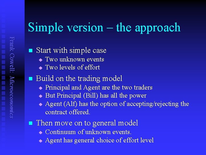
Simple version – the approach Frank Cowell: Microeconomics n Start with simple case u u n Build on the trading model u u u n Two unknown events Two levels of effort Principal and Agent are the two traders But Principal (Bill) has all the power Agent (Alf) has the option of accepting/rejecting the contract offered. Then move on to general model u u Continuum of unknown events. Agent has general choice of effort level

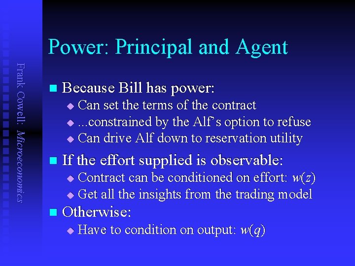
Power: Principal and Agent Frank Cowell: Microeconomics n Because Bill has power: Can set the terms of the contract u. . . constrained by the Alf’s option to refuse u Can drive Alf down to reservation utility u n If the effort supplied is observable: Contract can be conditioned on effort: w(z) u Get all the insights from the trading model u n Otherwise: u Have to condition on output: w(q)

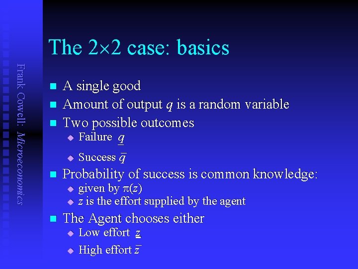
The 2 2 case: basics Frank Cowell: Microeconomics n n n A single good Amount of output q is a random variable Two possible outcomes u u n Probability of success is common knowledge: u u n Failure q –_ Success q given by p(z) z is the effort supplied by the agent The Agent chooses either u u Low effort z _ High effort z

The 2 2 case: motivation Frank Cowell: Microeconomics n The Agent's utility derives from u u u n The Agent is risk averse u n xb = q – xa (In the simple model) Principal is risk neutral u n ua( • , • ) is strictly concave in its first argument The Principal consumes all output not consumed by Agent u n consumption of the single good xa ( ) the effort put in, z ( ) Given v. NM preferences utility is Eua(xa, z). Utility is Eq – xa Can interpret this in the trading diagram

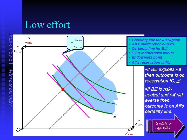
Low effort Frank Cowell: Microeconomics b x. RED a x. BLUE p. RED – ____ p. BLUE § Certainty line for Alf (Agent) b § Alf's curves Ob indifference O § Certainty line for Bill § Bill's indifference curves § Endowment point § Alf's reservation utility §If Bill exploits Alf then outcome is on reservation IC, ua §If Bill is riskneutral and Alf risk averse then outcome is on Alf's certainty line. ua b x. BLUE Oa a x. RED Switch to high effort

High effort Frank Cowell: Microeconomics b x. RED a x. BLUE p. RED – ____ p. BLUE § Certainty line and indifference curves forb Alf O Obb O § Certainty line and indifference curves for Bill § Endowment point § Alf's reservation utility §High effort tilts the ICs, shifts the equilibrium outcome. §Contrast with low effort b x. BLUE Oa a x. RED Combine to get menu of contracts

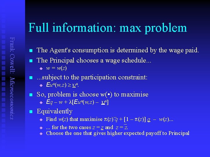
Full information: max problem Frank Cowell: Microeconomics n n The Agent's consumption is determined by the wage paid. The Principal chooses a wage schedule. . . u n . . . subject to the participation constraint: u n Eua(w, z) ua. So, problem is choose w( • ) to maximise u n w = w (z ) Eq – w + l[Eua (w, z) – ua ] Equivalently u u u _ Find w(z) that maximise p(z) q + _[1 – p(z)] q – w(z). . . for the two cases z = z and z = z. Choose the one that gives higher expected payoff to Principal

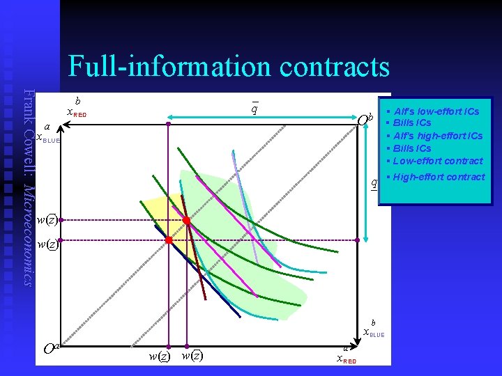
Full-information contracts Frank Cowell: Microeconomics – q b x. RED Ob a x. BLUE § Alf's low-effort ICs § Bills ICs § Alf's high-effort ICs § Bills ICs § Low-effort contract q § High-effort contract – – w(z) – b x. BLUE Oa – w(z) – a x. RED

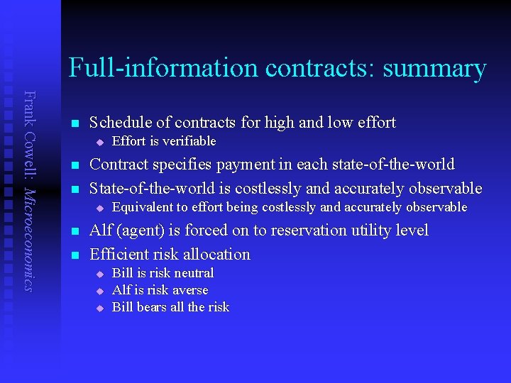
Full-information contracts: summary Frank Cowell: Microeconomics n Schedule of contracts for high and low effort u n n Contract specifies payment in each state-of-the-world State-of-the-world is costlessly and accurately observable u n n Effort is verifiable Equivalent to effort being costlessly and accurately observable Alf (agent) is forced on to reservation utility level Efficient risk allocation u u u Bill is risk neutral Alf is risk averse Bill bears all the risk

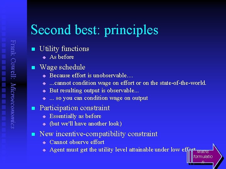
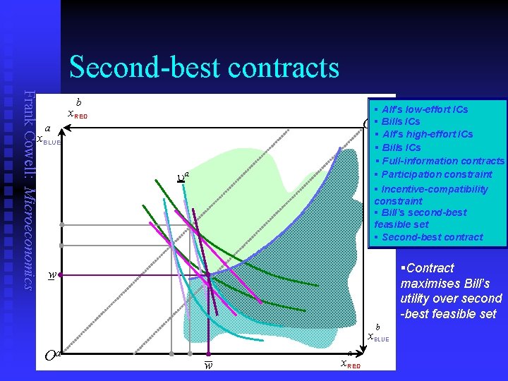
Second best: principles Frank Cowell: Microeconomics n Utility functions u n Wage schedule u u n Because effort is unobservable…. . . cannot condition wage on effort or on the state-of-the-world. But resulting output is observable. . . so you can condition wage on output Participation constraint u u n As before Essentially as before (but we'll have another look) New incentive-compatibility constraint u u Cannot observe effort Agent must get the utility level attainable under low effort Maths formulatio n

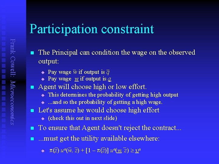
Participation constraint Frank Cowell: Microeconomics n The Principal can condition the wage on the observed output: u u n Agent will choose high or low effort. u u n n This determines the probability of getting high output. . . and so the probability of getting a high wage. Let's assume he would choose high effort u n _ _ Pay wage w if output is q (check this out in next slide) To ensure that Agent doesn't reject the contract. . . must get the utility available elsewhere: u _ _ _ a a p(z) u (w, z) + [1 – p(z)] u (w, z) ua

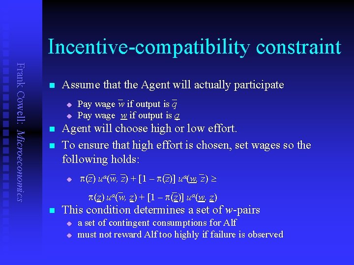
Incentive-compatibility constraint Frank Cowell: Microeconomics n Assume that the Agent will actually participate u u n n Agent will choose high or low effort. To ensure that high effort is chosen, set wages so the following holds: u n _ _ Pay wage w if output is q _ _ _ a a p(z) u (w, z) + [1 – p(z)] u (w, z) _ _ a p(z) u (w, z) + [1 – p(z)] ua (w, z) This condition determines a set of w-pairs u u a set of contingent consumptions for Alf must not reward Alf too highly if failure is observed

Second-best contracts Frank Cowell: Microeconomics b § Alf's low-effort ICs Ob§ Bills ICs § Alf's high-effort ICs § Bills ICs § Full-information contracts § Participation constraint § Incentive-compatibility constraint § Bill’s second-best feasible set § Second-best contract x. RED a x. BLUE ua §Contract maximises Bill’s utility over second -best feasible set –w b x. BLUE Oa – w a x. RED

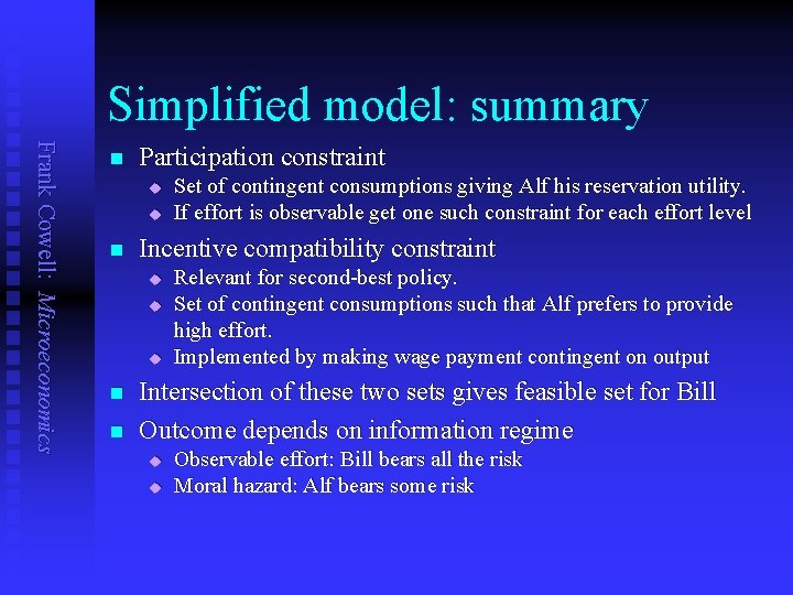
Simplified model: summary Frank Cowell: Microeconomics n Participation constraint u u n Incentive compatibility constraint u u u n n Set of contingent consumptions giving Alf his reservation utility. If effort is observable get one such constraint for each effort level Relevant for second-best policy. Set of contingent consumptions such that Alf prefers to provide high effort. Implemented by making wage payment contingent on output Intersection of these two sets gives feasible set for Bill Outcome depends on information regime u u Observable effort: Bill bears all the risk Moral hazard: Alf bears some risk

Overview. . . Moral Hazard Frank Cowell: Microeconomics The basics Extending the “first-order” approach A simplified model The general model

General model: introduction Frank Cowell: Microeconomics n Retain assumption that it is a two-person contest. u u u n Again deal with full-information case first. u u n Same roles for Principal and Agent. But… Allow for greater range of choice for Agent Allow for different preferences for Principal Draw on lessons from 2× 2 case Same principles apply Then introduce the possibility of unobserved effort. u u Needs some modification from 2× 2 case But similar principles emerge

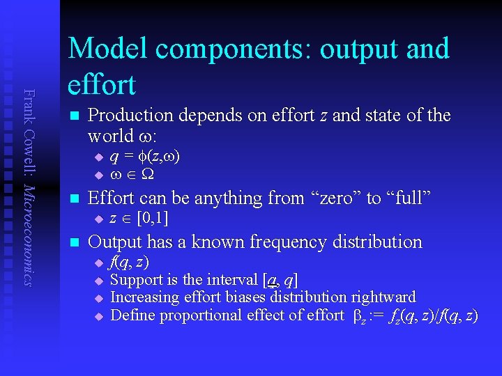
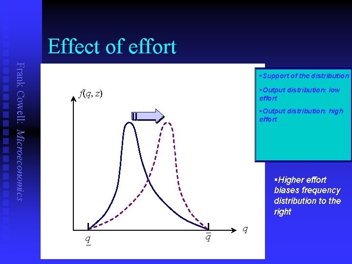
Frank Cowell: Microeconomics Model components: output and effort n Production depends on effort z and state of the world w: u u n Effort can be anything from “zero” to “full” u n q = f(z, w) w W z [0, 1] Output has a known frequency distribution u u f(q, z) Support is the interval [q, q] Increasing effort biases distribution rightward Define proportional effect of effort bz : = fz (q, z)/f(q, z)

Effect of effort Frank Cowell: Microeconomics §Support of the distribution §Output distribution: low effort f(q, z) §Output distribution: high effort §Higher effort biases frequency distribution to the right q – q– q

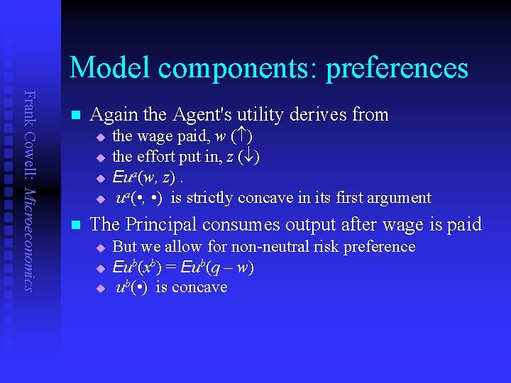
Model components: preferences Frank Cowell: Microeconomics n Again the Agent's utility derives from u u n the wage paid, w ( ) the effort put in, z ( ) Eua (w, z). ua( • , • ) is strictly concave in its first argument The Principal consumes output after wage is paid u u u But we allow for non-neutral risk preference Eub(xb) = Eub(q – w) ub ( • ) is concave

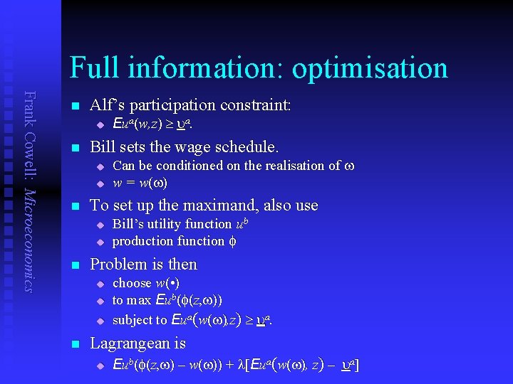
Full information: optimisation Frank Cowell: Microeconomics n Alf’s participation constraint: u n Bill sets the wage schedule. u u n u Bill’s utility function ub production function f Problem is then u u u n Can be conditioned on the realisation of w w = w (w ) To set up the maximand, also use u n Eua(w, z) ua. choose w( • ) to max Eub(f(z, w)) subject to Eua(w(w), z) ua. Lagrangean is u Eub(f(z, w) – w(w)) + l[Eua(w(w), z) – ua]

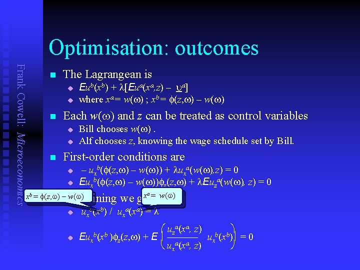
Optimisation: outcomes Frank Cowell: Microeconomics n The Lagrangean is u u n Each w(w) and z can be treated as control variables u u n Eub(xb) + l[Eua(xa, z) – ua] where xa = w(w) ; xb = f(z, w) – w(w) Bill chooses w(w). Alf chooses z, knowing the wage schedule set by Bill. First-order conditions are u u – uxb(f(z, w) – w(w)) + luxa(w(w), z) = 0 Euxb(f(z, w) – w(w))fz(z, w) + l. Euza(w(w), z) = 0 xb = f(z, w) w(w) n –Combining u u x = we get a w(w) uxb (xb ) / uxa (xa ) = l uza(xa, z) b b Eux (x )fz (z, w) + E ux (x ) = 0 uxa(xa, z)

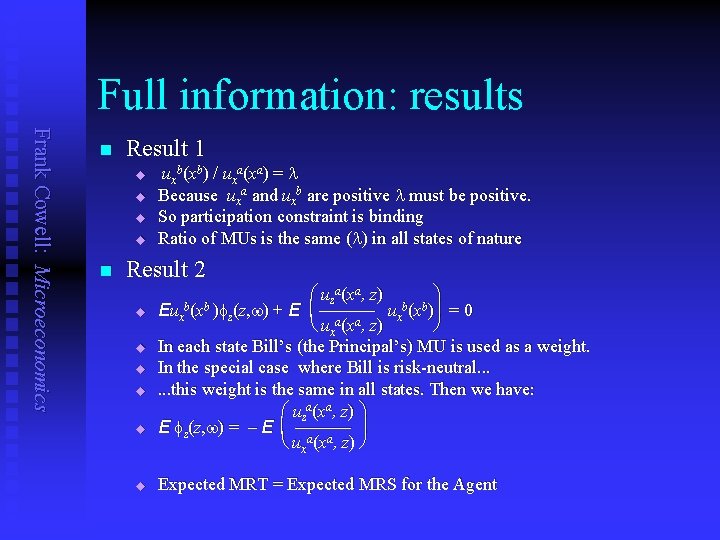
Full information: results Frank Cowell: Microeconomics n Result 1 u u n uxb(xb) / uxa(xa) = l Because uxa and uxb are positive l must be positive. So participation constraint is binding Ratio of MUs is the same (l) in all states of nature Result 2 u u u uza(xa, z) b b Eux (x )fz (z, w) + E ux (x ) = 0 uxa(xa, z) In each state Bill’s (the Principal’s) MU is used as a weight. In the special case where Bill is risk-neutral. . . this weight is the same in all states. Then we have: uza (xa , z) E fz(z, w) = – E uxa (xa , z) Expected MRT = Expected MRS for the Agent

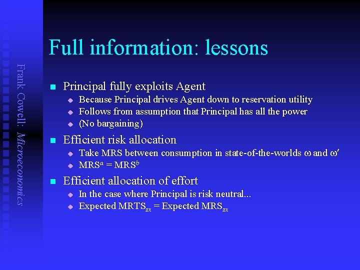
Full information: lessons Frank Cowell: Microeconomics n Principal fully exploits Agent u u u n Efficient risk allocation u u n Because Principal drives Agent down to reservation utility Follows from assumption that Principal has all the power (No bargaining) Take MRS between consumption in state-of-the-worlds w and w MRSa = MRSb Efficient allocation of effort u u In the case where Principal is risk neutral. . . Expected MRTSzx = Expected MRSzx

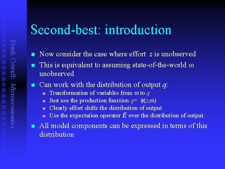
Second-best: introduction Frank Cowell: Microeconomics n n n Now consider the case where effort z is unobserved This is equivalent to assuming state-of-the-world w unobserved Can work with the distribution of output q: u u n Transformation of variables from w to q Just use the production function q= f(z, w) Clearly effort shifts the distribution of output Use the expectation operator E over the distribution of output. All model components can be expressed in terms of this distribution

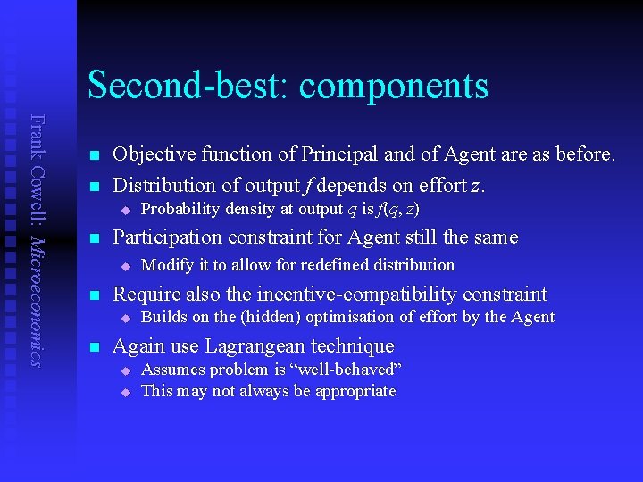
Second-best: components Frank Cowell: Microeconomics n n Objective function of Principal and of Agent are as before. Distribution of output f depends on effort z. u n Participation constraint for Agent still the same u n Modify it to allow for redefined distribution Require also the incentive-compatibility constraint u n Probability density at output q is f(q, z) Builds on the (hidden) optimisation of effort by the Agent Again use Lagrangean technique u u Assumes problem is “well-behaved” This may not always be appropriate

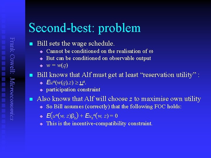
Second-best: problem Frank Cowell: Microeconomics n Bill sets the wage schedule. u u u n Bill knows that Alf must get at least “reservation utility” : u u n Cannot be conditioned on the realisation of w But can be conditioned on observable output w = w(q) Eua(w(q), z) ua. participation constraint Also knows that Alf will choose z to maximise own utility u u u So Bill assumes (correctly) that the following FOC holds: E(ua(w, z)bz) + Euza(w, z) = 0 This is the incentive-compatibility constraint.

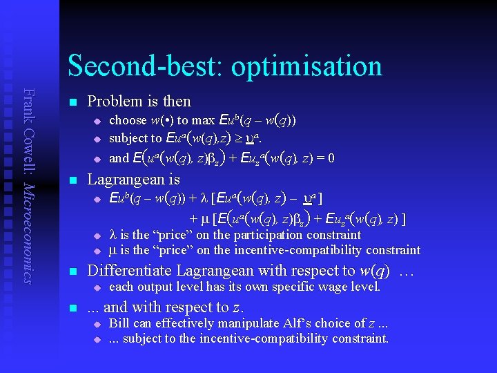
Second-best: optimisation Frank Cowell: Microeconomics n Problem is then u u u n Lagrangean is u Eub(q – w(q)) + l [Eua(w(q), z) – ua ] + m [E(ua(w(q), z)bz) + Euza(w(q), z) ] u u n l is the “price” on the participation constraint m is the “price” on the incentive-compatibility constraint Differentiate Lagrangean with respect to w(q) … u n choose w( • ) to max Eub(q – w(q)) subject to Eua(w(q), z) ua. and E(ua(w(q), z)bz) + Euza(w(q), z) = 0 each output level has its own specific wage level. . and with respect to z. u u Bill can effectively manipulate Alf’s choice of z. . . subject to the incentive-compatibility constraint.

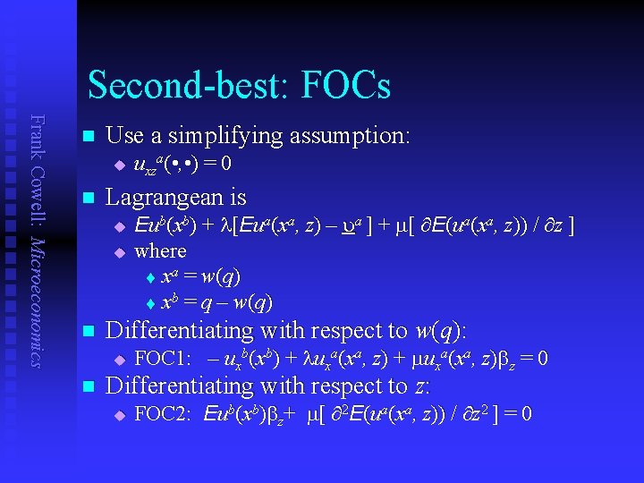
Second-best: FOCs Frank Cowell: Microeconomics n Use a simplifying assumption: u n Lagrangean is u u n Eub(xb) + l[Eua(xa, z) – ua ] + m[ E(ua(xa, z)) / z ] where t xa = w(q) t xb = q – w(q) Differentiating with respect to w(q): u n uxza( • , • ) = 0 FOC 1: – uxb(xb) + luxa(xa, z) + muxa(xa, z)bz = 0 Differentiating with respect to z: u FOC 2: Eub(xb)bz+ m[ 2 E(ua(xa, z)) / z 2 ] = 0

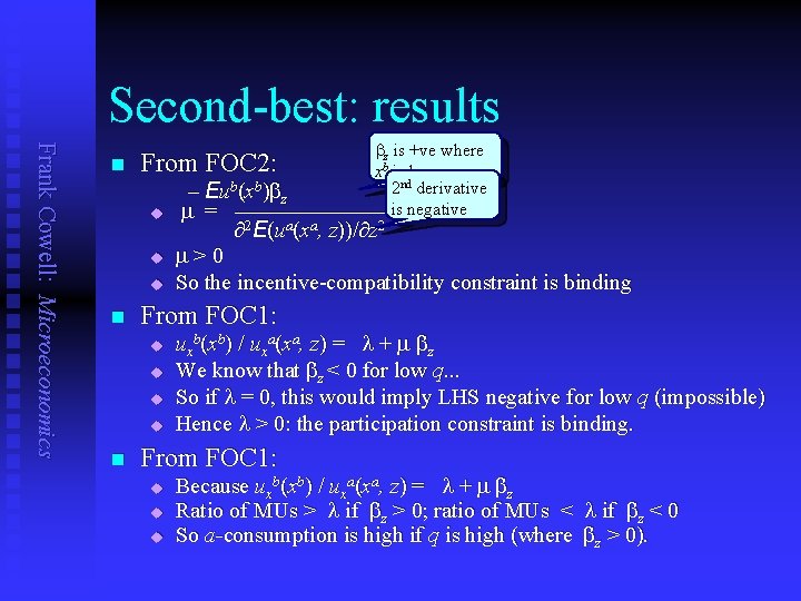
Second-best: results Frank Cowell: Microeconomics bz is +ve where n From FOC 2: xb is large 2 nd derivative – Eub(xb)bz u m = ———————is negative 2 E(ua(xa, z))/ z 2 u u n From FOC 1: u u n m>0 So the incentive-compatibility constraint is binding uxb(xb) / uxa(xa, z) = l + m bz We know that bz < 0 for low q. . . So if l = 0, this would imply LHS negative for low q (impossible) Hence l > 0: the participation constraint is binding. From FOC 1: u u u Because uxb(xb) / uxa(xa, z) = l + m bz Ratio of MUs > l if bz > 0; ratio of MUs < l if bz < 0 So a-consumption is high if q is high (where bz > 0).

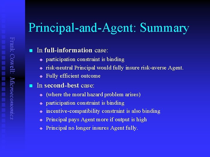
Principal-and-Agent: Summary Frank Cowell: Microeconomics n In full-information case: u u u n participation constraint is binding risk-neutral Principal would fully insure risk-averse Agent. Fully efficient outcome In second-best case: u u u (where the moral hazard problem arises) participation constraint is binding incentive-compatibility constraint is also binding Principal pays Agent more if output is high Principal no longer insures Agent fully.