Flow Visualization MJ Turner MSc ACS COMP 60051

Flow Visualization MJ Turner MSc ACS COMP 60051 Manchester

Overview § § § Classes of data: scalar, vector, tensor Introduction to experimental flow visualization Some techniques described Double Glazing case study Conclusions and summary 2 Flow/03 2

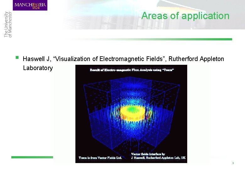
Areas of application § Haswell J, “Visualization of Electromagnetic Fields”, Rutherford Appleton Laboratory 2 Flow/03 3

Other Application Areas § § § Design of cars, aircraft, ships, submarines & spacecraft Design of the components: turbines, combustion engines Flow inside blood vessels River and ocean flow Wind effects between buildings 2 Flow/03 4

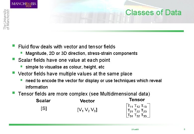
Classes of Data § § § Fluid flow deals with vector and tensor fields § Magnitude, 2 D or 3 D direction, stress-strain components Scalar fields have one value at each point § simple to visualise as colour, height, etc Vector fields have multiple values at the same place § need to encode the vector for display or use techniques which reveal § information Tensor fields are more complex (see Multidimensional data) 2 Flow/03 5

Experimental Visualization (without computers) § There are three main classes of technique § addition of foreign material § optical techniques § addition of heat and energy 2 Flow/03 6

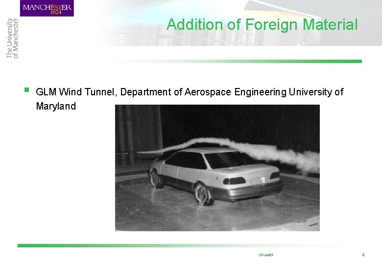
Addition of foreign material § § time lines: lines transformed by the motion of fluid flow § e. g. , a line of hydrogen bubbles streak lines: shows the motion by injecting a dye from a fixed position for a defined time § e. g. , dye in fluid, smoke in air path line: path of a particle introduced into the flow § e. g. , exposure of photographic plate to light emitting particle For flow over surfaces § e. g. , direction of tufts fixed to the surface or traces left by viscous fluid on surface 2 Flow/03 7

Addition of Foreign Material § GLM Wind Tunnel, Department of Aerospace Engineering University of Maryland 2 Flow/03 8

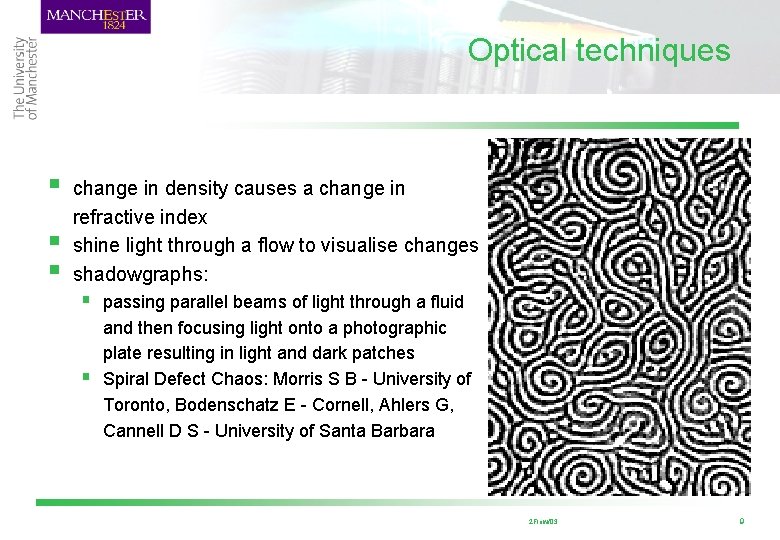
Optical techniques § § § change in density causes a change in refractive index shine light through a flow to visualise changes shadowgraphs: § passing parallel beams of light through a fluid § and then focusing light onto a photographic plate resulting in light and dark patches Spiral Defect Chaos: Morris S B - University of Toronto, Bodenschatz E - Cornell, Ahlers G, Cannell D S - University of Santa Barbara 2 Flow/03 9

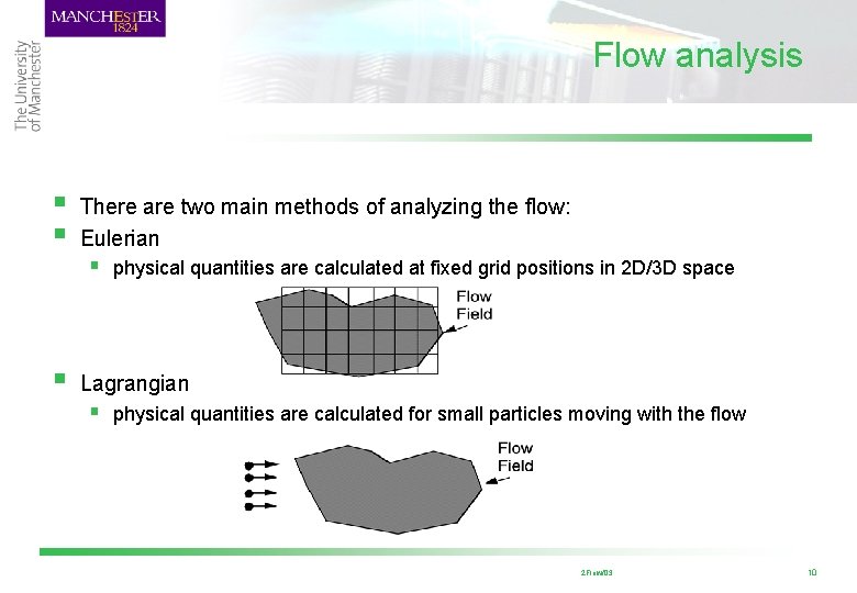
Flow analysis § § There are two main methods of analyzing the flow: Eulerian § physical quantities are calculated at fixed grid positions in 2 D/3 D space § Lagrangian § physical quantities are calculated for small particles moving with the flow 2 Flow/03 10

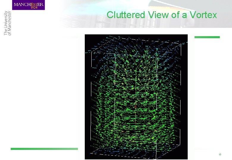
Arrow Plots (Hedgehogs) § § § Arrow icon at each grid point (Eulerian analysis) § Magnitude maps to arrow length § Direction maps to shaft direction Useful in 2 D provided grid points not closely spaced Bad problem of occlusion in 3 D Susceptible to artefacts because of the spurious high-frequency detail Gives behaviour at point samples, not behaviour of the field as a whole 2 Flow/03 11

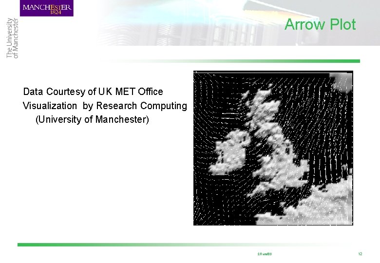
Arrow Plot Data Courtesy of UK MET Office Visualization by Research Computing (University of Manchester) 2 Flow/03 12

Cluttered View of a Vortex 2 Flow/03 13

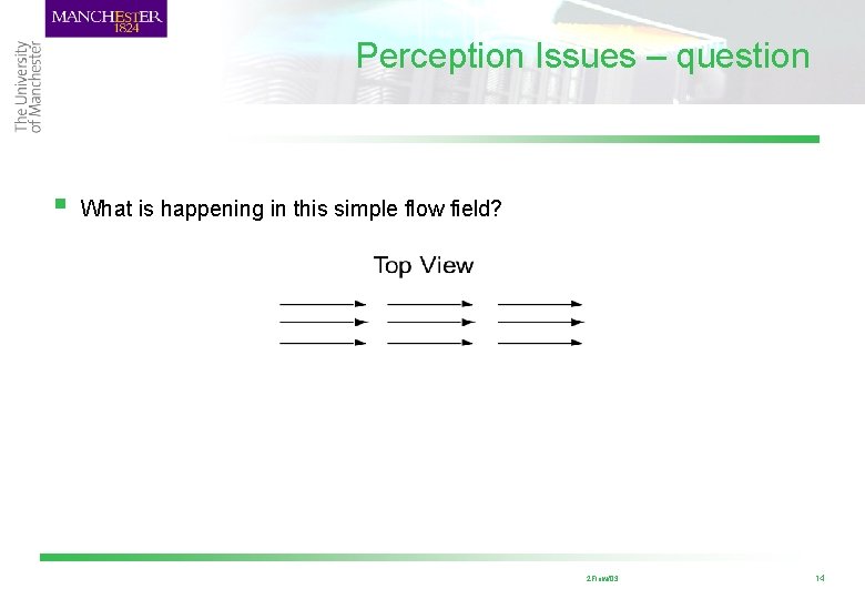
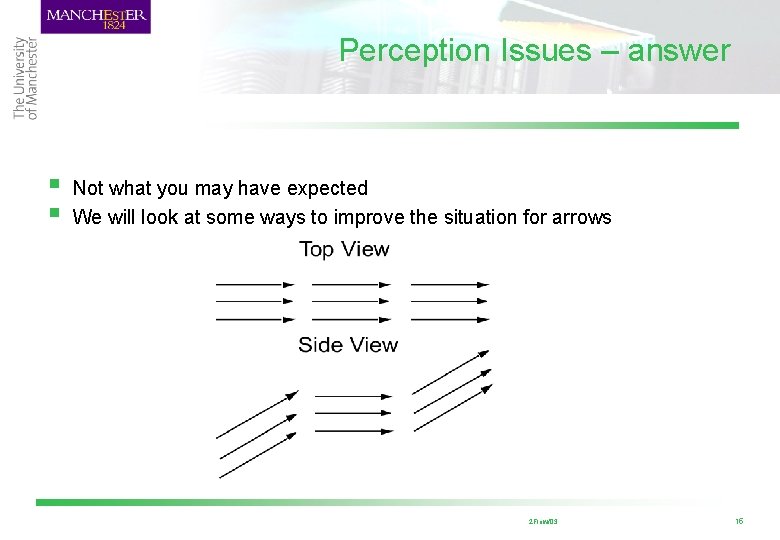
Perception Issues – question § What is happening in this simple flow field? 2 Flow/03 14

Perception Issues – answer § § Not what you may have expected We will look at some ways to improve the situation for arrows 2 Flow/03 15

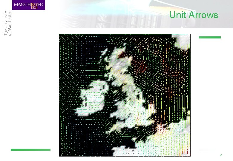
Unit Arrow (hedgehog) fields § § § Arrow shafts all same length § reduces orientation ambiguity § less occlusion Gives information about direction of vectors No information on magnitude, but this can be added: § Shaft or arrowhead colour 2 Flow/03 16

Unit Arrows 2 Flow/03 17

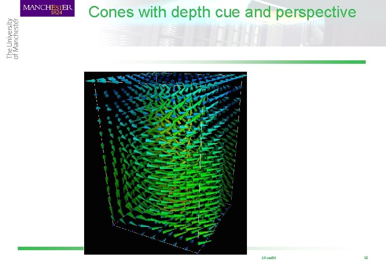
Shadowed hedgehog fields § § § Use with either plain or unit hedgehogs Best with 2 D domain Shadows cast onto plane help show orientation Depth cueing of arrows can also reduce orientation ambiguity Instead of arrows you could use other geometric objects which themselves offer more visual cues e. g. , cones 2 Flow/03 18

Cones with depth cue and perspective 2 Flow/03 19

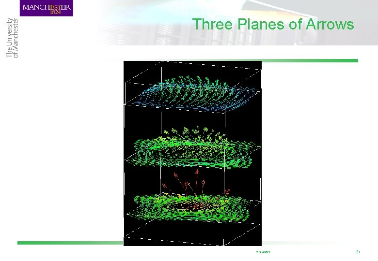
Subsetting the domain § § § Probe shows point behaviour Rake of probes shows behaviour at intervals § limits number of arrows seen at once Slicing plane views a 2 D slice of a 3 D domain § extra dimension freed to represent another parameter § Interactive positioning and adjustment allows exploration of interesting regions 2 Flow/03 20

Three Planes of Arrows 2 Flow/03 21

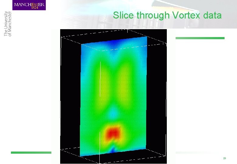
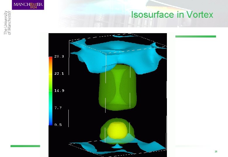
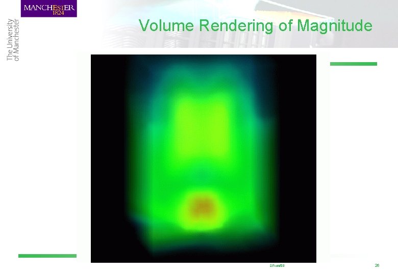
Convert vectors to scalars § § § Simplest possible method Extract a scalar: § Single component (x, y, z) of a vector is rarely useful § Vector magnitude – good overview of a field § Divergence can be interesting Visualise using standard scalar techniques: § § colour on a vector technique Slicing Isosurface volume rendering 2 Flow/03 22

Slice through Vortex data 2 Flow/03 23

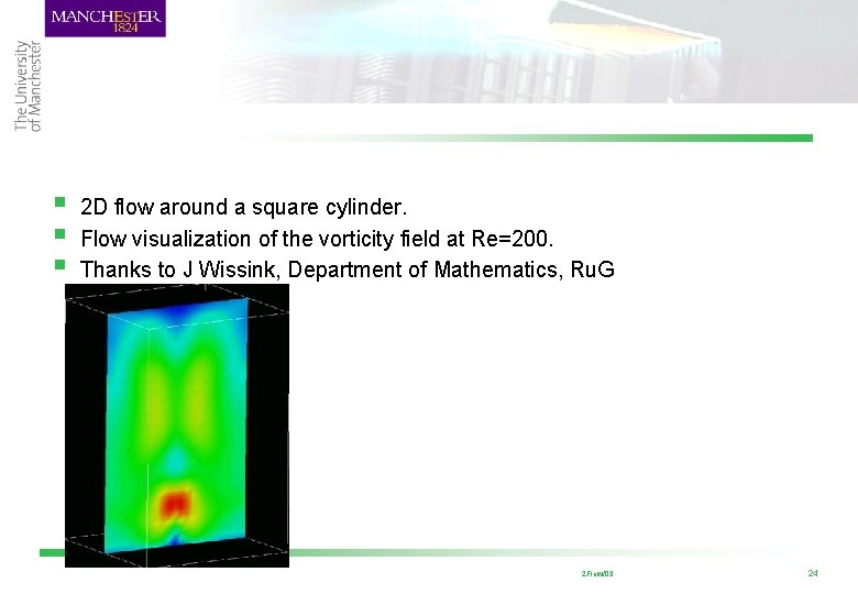
§ § § 2 D flow around a square cylinder. Flow visualization of the vorticity field at Re=200. Thanks to J Wissink, Department of Mathematics, Ru. G 2 Flow/03 24

Isosurface in Vortex 2 Flow/03 25

Volume Rendering of Magnitude 2 Flow/03 26

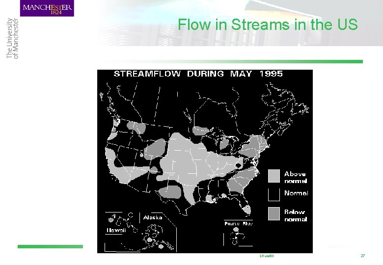
Flow in Streams in the US 2 Flow/03 27

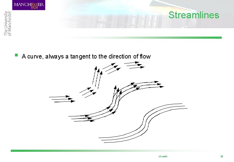
Streamlines § A curve, always a tangent to the direction of flow 2 Flow/03 28

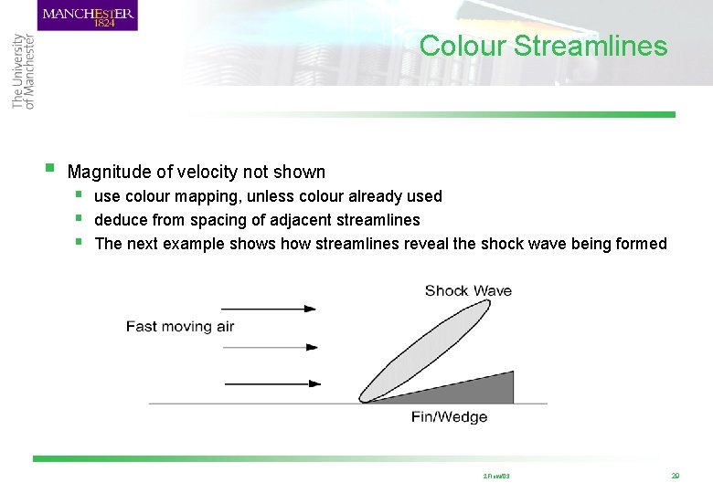
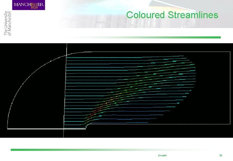
Colour Streamlines § Magnitude of velocity not shown § use colour mapping, unless colour already used § deduce from spacing of adjacent streamlines § The next example shows how streamlines reveal the shock wave being formed 2 Flow/03 29

Coloured Streamlines § See notes for picture 2 Flow/03 30

Perceptual Issues § § Problem of occlusion, if lots of them § adjust viewpoint or use clipping planes Perception problem with 3 D location § § use depth cueing by hue or saturation add colouring by height or depth use stereoscopic or immersive VR to aid location A list of sites can be found under http: //ccf. arc. nasa. gov/ra/page 3. html 2 Flow/03 31

NASA Ames Virtual Wind Tunnel [6] 2 Flow/03 32

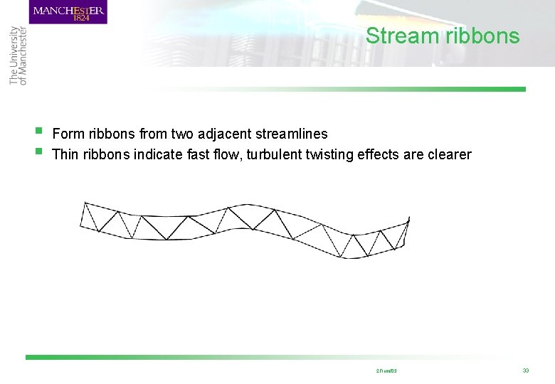
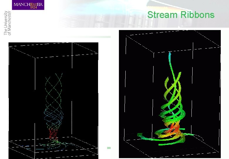
Stream ribbons § § Form ribbons from two adjacent streamlines Thin ribbons indicate fast flow, turbulent twisting effects are clearer 2 Flow/03 33

Stream Ribbons 2 Flow/03 34

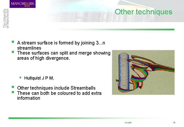
Other techniques § § A stream surface is formed by joining 3. . . n streamlines These surfaces can split and merge showing areas of high divergence. § Hultquist J P M, § § Other techniques include Streamballs These can both be coloured to add extra information 2 Flow/03 35

Particle advection

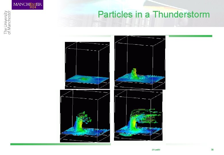
Streak and path lines § § § These are directly related to the experimental counterpart Another common name for path lines are particle traces They are usually shown as animated sequences: § a single instance in an unsteady flow § over a defined time interval in a steady flow 2 Flow/03 37

Particles in a Thunderstorm 2 Flow/03 38

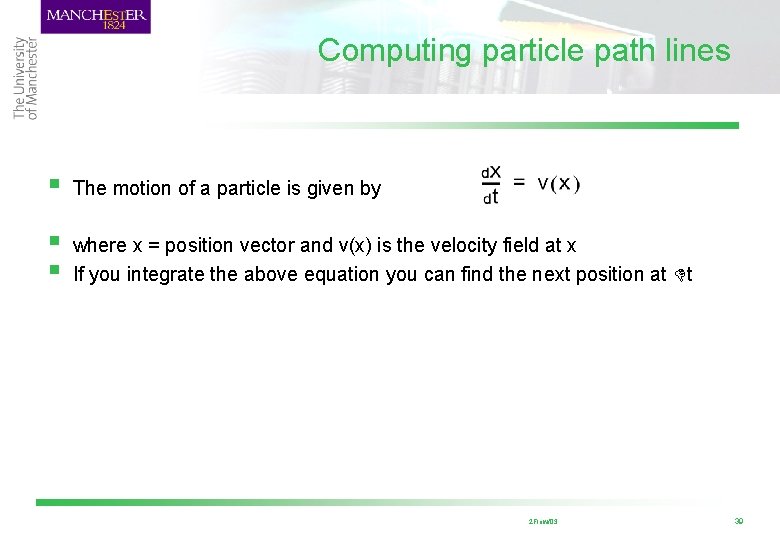
Computing particle path lines § The motion of a particle is given by § § where x = position vector and v(x) is the velocity field at x If you integrate the above equation you can find the next position at t 2 Flow/03 39

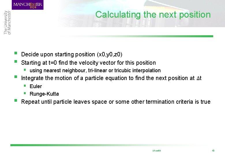
Calculating the next position § § Decide upon starting position (x 0, y 0, z 0) Starting at t=0 find the velocity vector for this position § using nearest neighbour, tri-linear or tricubic interpolation Integrate the motion of a particle equation to find the next position at ∆t § Euler § Runge-Kutta Repeat until particle leaves space or some other termination criteria is true 2 Flow/03 40

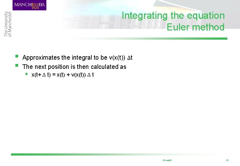
Integrating the equation Euler method § § Approximates the integral to be v(x(t)) ∆t The next position is then calculated as § x(t+ ∆ t) = x(t) + v(x(t)) ∆ t 2 Flow/03 41

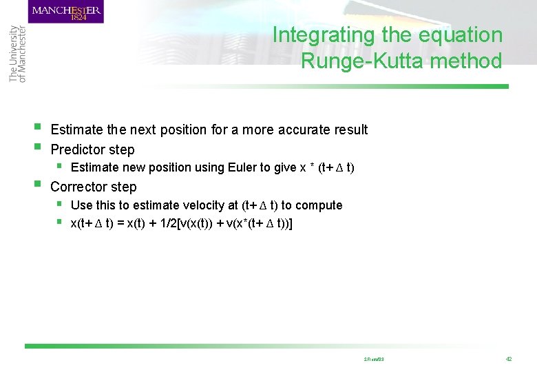
Integrating the equation Runge-Kutta method § § Estimate the next position for a more accurate result Predictor step § Corrector step § Estimate new position using Euler to give x * (t+ ∆ t) § Use this to estimate velocity at (t+ ∆ t) to compute § x(t+ ∆ t) = x(t) + 1/2[v(x(t)) + v(x*(t+ ∆ t))] 2 Flow/03 42

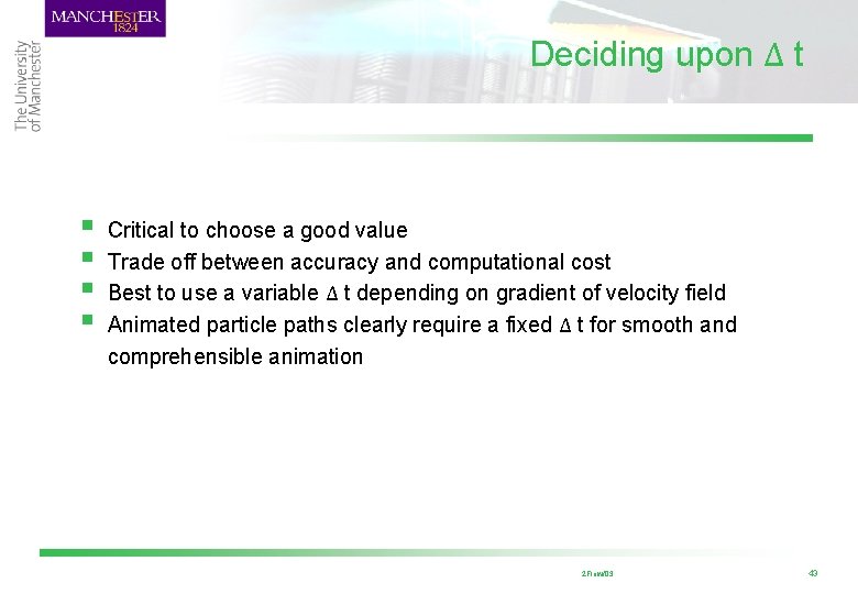
Deciding upon ∆ t § § Critical to choose a good value Trade off between accuracy and computational cost Best to use a variable ∆ t depending on gradient of velocity field Animated particle paths clearly require a fixed ∆ t for smooth and comprehensible animation 2 Flow/03 43

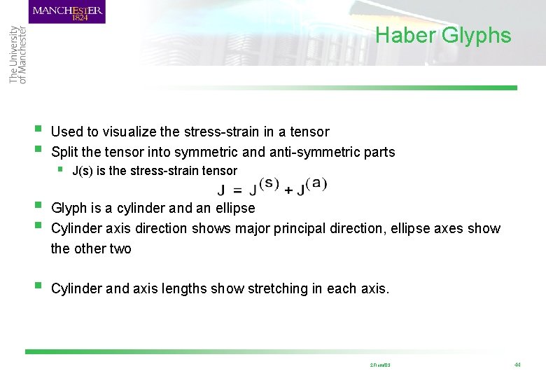
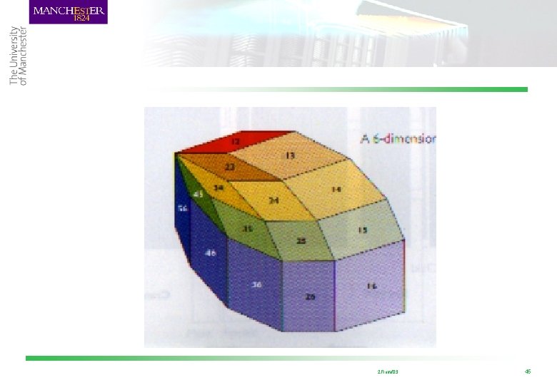
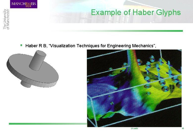
Haber Glyphs § § Used to visualize the stress-strain in a tensor Split the tensor into symmetric and anti-symmetric parts § J(s) is the stress-strain tensor § § Glyph is a cylinder and an ellipse Cylinder axis direction shows major principal direction, ellipse axes show the other two § Cylinder and axis lengths show stretching in each axis. 2 Flow/03 44

2 Flow/03 45

Example of Haber Glyphs § Haber R B, “Visualization Techniques for Engineering Mechanics”, 2 Flow/03 46

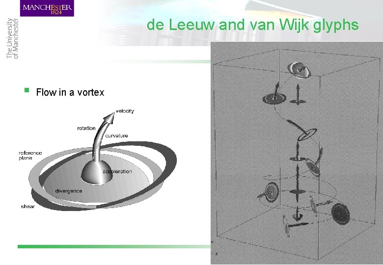
de Leeuw and van Wijk glyphs § § § Visualise the tensor field in the context of the associated velocity field Steady state flows only Best used as a probe or small multiple Constructs local coordinate axis as with Haber glyphs Decompose tensor into parallel & perpendicular components Extract further components from these § acceleration, shear, curvature (parallel) § torsion, divergence (perpendicular) 2 Flow/03 47

de Leeuw and van Wijk glyphs § Flow in a vortex 2 Flow/03 48

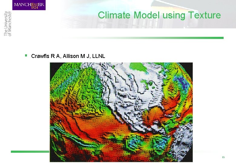
Textures § § § In addition to surface height, colour and vectors we can use texture (bump mapping) Bump map is a collection of bumps (texture) used to additional information to a graphical primitive Interactive adjustment of parameters is desirable to obtain best results Careful use is needed as additions to an already rough surface can be distracting 2 Flow/03 49

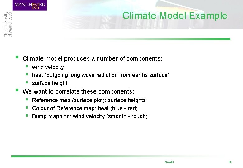
Climate Model Example § § Climate model produces a number of components: § wind velocity § heat (outgoing long wave radiation from earths surface) § surface height We want to correlate these components: § Reference map (surface plot): surface heights § Colour of Reference map: heat (blue - red) § Bump mapping: wind velocity (smooth - rough) 2 Flow/03 50

Climate Model using Texture § Crawfis R A, Allison M J, LLNL 2 Flow/03 51

More use of textures § § § Texture maps can be used to represent more information about vectors and tensors than just magnitude The process is called “Line Integral Convolution” You take: § a vector field defined on a cartesian grid § a texture map of the same dimensions “The output image is a one-one correspondence of a 1 D convolution of a filter kernal and texture pixels along a local streamline in the vector field” More simply the texture is “smeared” in the direction of the vector field 2 Flow/03 52

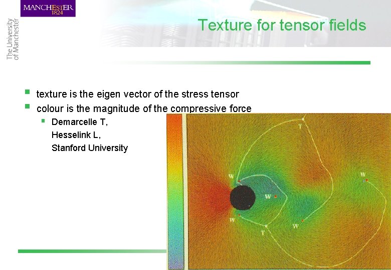
Texture for tensor fields § § texture is the eigen vector of the stress tensor colour is the magnitude of the compressive force § Demarcelle T, Hesselink L, Stanford University 2 Flow/03 53

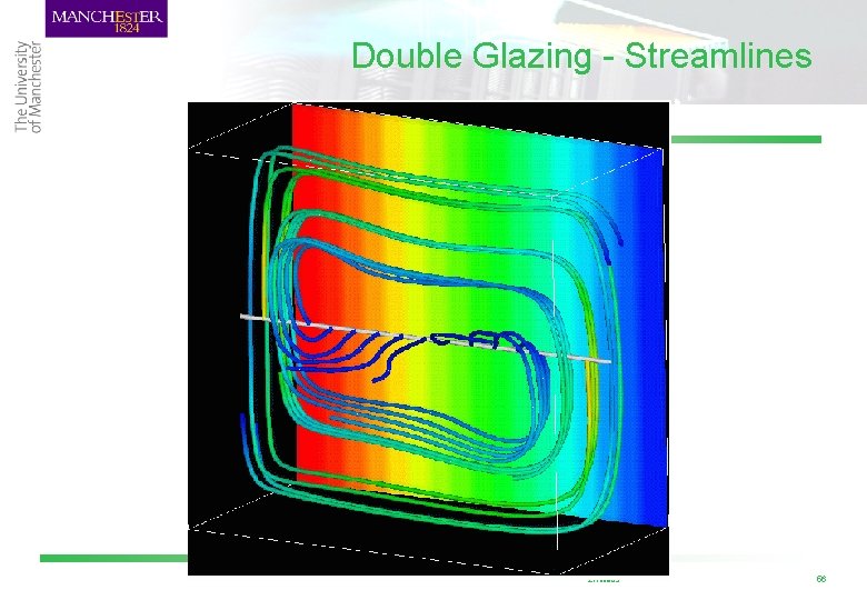
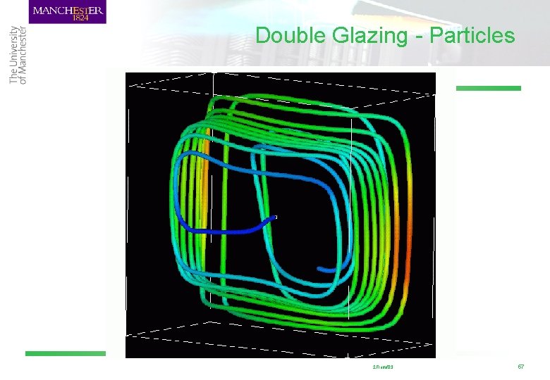
Double Glazing Case Study § § The dataset and observations came from Dr Tim David, Mechanical Engineering Department, University of Leeds It is a study of the behaviour of air flow between two plates, where one plate is cold and the other is warm e. g. , double glazing There is a linear temperature variation between the two plates § See notes for picture § 2 Flow/03 54

Double Glazing – Arrows § See notes 2 Flow/03 55

Double Glazing - Streamlines 2 Flow/03 56

Double Glazing - Particles 2 Flow/03 57

Systems § Most of the current Visualization Environments support the major flow visualization techniques: § Application Visualization System (AVS) § IBM Data Explorer § Iris Explorer § More limited techniques are available in Khoros, PV-Wave, IDL 2 Flow/03 58

More Systems § Other turnkey/public domain systems with extra features for flow visualization: § Data Visualiser § FAST: NASA Ames (http: //www. nasa. gov/FAST/fast. html) , § ISVAS: research prototype developed by Fraunhofer Institute for Computer § Graphics Darmstadt, Germany (ftp: //ftp. igd. fhg. de: pub/isvas) Visual 3: (http: //raphael. mit. edu/visual 3. html) 2 Flow/03 59

Conclusions § § The techniques are very useful for 2 D flow. We can represent single 3 D vectors but we ideally want to visualize the 3 D flow field Lot of current research in methods to represent fields of vectors and some of these include § Direct volume rendering § Stream surfaces with additional cues § Area glyphs to summarise characteristics We will see some of these in the section on Multidimensional data 2 Flow/03 60