Exploring Microsoft Office 2016 Series Editor Mary Anne

Exploring Microsoft® Office 2016 Series Editor Mary Anne Poatsy Mulbery|Krebs|Hogan|Cameron |Davidson|Lau|Lawson|Williams Series Created by Dr. Robert T. Grauer

Exploring Excel 2016 Chapter 2 Copyright © 2017 Pearson Education, Inc.

Objective 1: Use Relative, Absolute, and Mixed Cell References in Formulas Skills: Use a Relative Cell Reference Use an Absolute Cell Reference Use a Mixed Cell Reference Copyright © 2017 Pearson Education, Inc.

Use Relative, Absolute, and Mixed Cell References in Formulas • When we build a formula, we use cell references, such as =B 2*B 3. • Excel uses three different ways to reference a cell in a formula: relative, absolute, and mixed. Copyright © 2017 Pearson Education, Inc.

Use Relative, Absolute, and Mixed Cell References in Formulas • Relative cell reference • A relative cell reference indicates a cell’s relative location, such as five rows up and one column to the left, from the cell containing the formula. • When you copy a formula containing a relative cell reference, the cell references in the copied formula change relative to the position of the copied formula. • Regardless of where you copy the formula, the cell references in the copied formula maintain the same relative distance from the cell containing the copied formula. Copyright © 2017 Pearson Education, Inc.

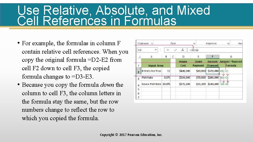
Use Relative, Absolute, and Mixed Cell References in Formulas • For example, the formulas in column F contain relative cell references. When you copy the original formula =D 2 -E 2 from cell F 2 down to cell F 3, the copied formula changes to =D 3 -E 3. • Because you copy the formula down the column to cell F 3, the column letters in the formula stay the same, but the row numbers change to reflect the row to which you copied the formula. Copyright © 2017 Pearson Education, Inc.

Use Relative, Absolute, and Mixed Cell References in Formulas • Absolute cell reference • An absolute cell reference provides a permanent reference to a specific cell. • When you copy a formula containing an absolute cell reference, the cell reference in the copied formula does not change, regardless of where you copy the formula. • An absolute cell reference appears with a dollar sign before both the column letter and row number, such as $B$4. Copyright © 2017 Pearson Education, Inc.

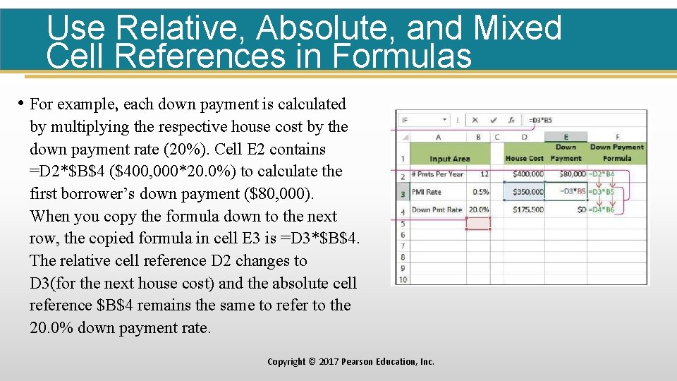
Use Relative, Absolute, and Mixed Cell References in Formulas • For example, each down payment is calculated by multiplying the respective house cost by the down payment rate (20%). Cell E 2 contains =D 2*$B$4 ($400, 000*20. 0%) to calculate the first borrower’s down payment ($80, 000). When you copy the formula down to the next row, the copied formula in cell E 3 is =D 3*$B$4. The relative cell reference D 2 changes to D 3(for the next house cost) and the absolute cell reference $B$4 remains the same to refer to the 20. 0% down payment rate. Copyright © 2017 Pearson Education, Inc.

Use Relative, Absolute, and Mixed Cell References in Formulas • Mixed cell reference • A mixed cell reference combines an absolute cell reference with a relative cell reference. • When you copy a formula containing a mixed cell reference, either the column letter or the row number that has the absolute reference remains fixed while the other part of the cell reference that is relative changes in the copied formula. Copyright © 2017 Pearson Education, Inc.

Use Relative, Absolute, and Mixed Cell References in Formulas • Mixed cell reference • $B 4 and B$4 are examples of mixed cell references. • In the reference $B 4, the column B is absolute, and the row number is relative; when you copy the formula, the column letter, B, does not change, but the row number will change. • In the reference B$4, the column letter, B, changes, but the row number, 4, does not change. To create a mixed reference, type the dollar sign to the left of the part of the cell reference you want to be absolute. Copyright © 2017 Pearson Education, Inc.

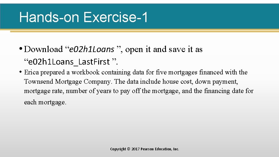
Hands-on Exercise-1 • Download “e 02 h 1 Loans ”, open it and save it as “e 02 h 1 Loans_Last. First ”. • Erica prepared a workbook containing data for five mortgages financed with the Townsend Mortgage Company. The data include house cost, down payment, mortgage rate, number of years to pay off the mortgage, and the financing date for each mortgage. Copyright © 2017 Pearson Education, Inc.

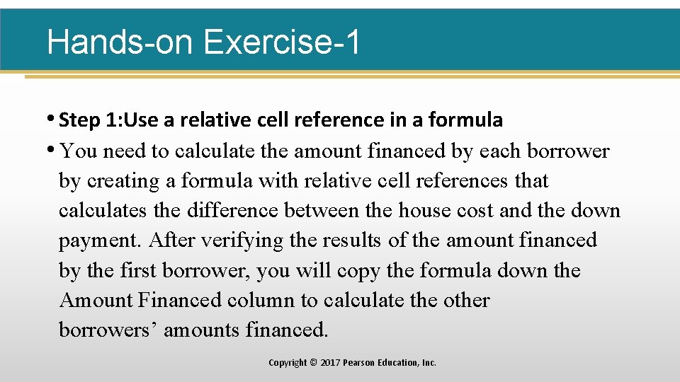
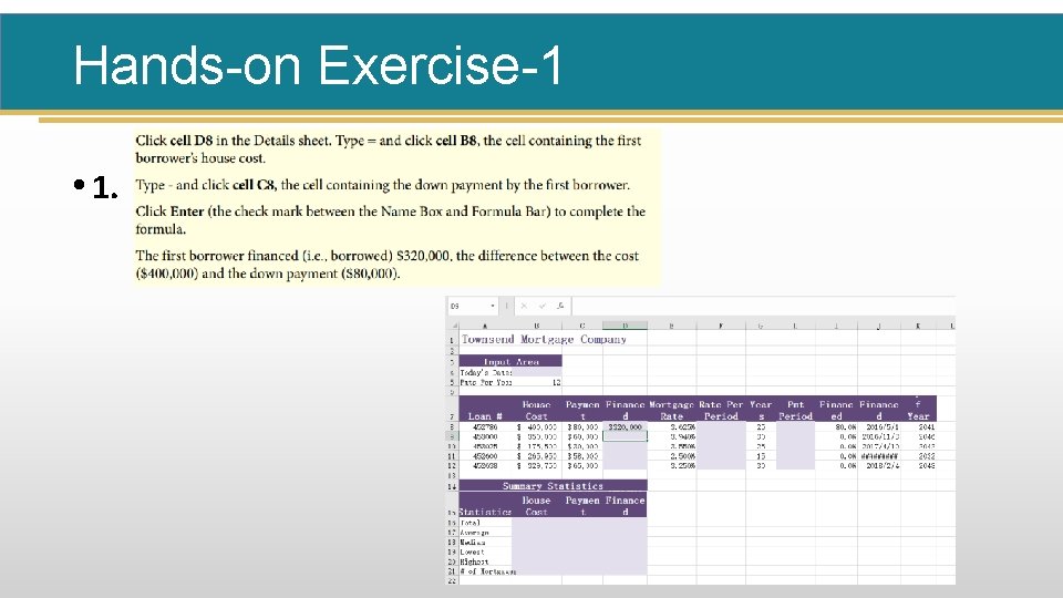
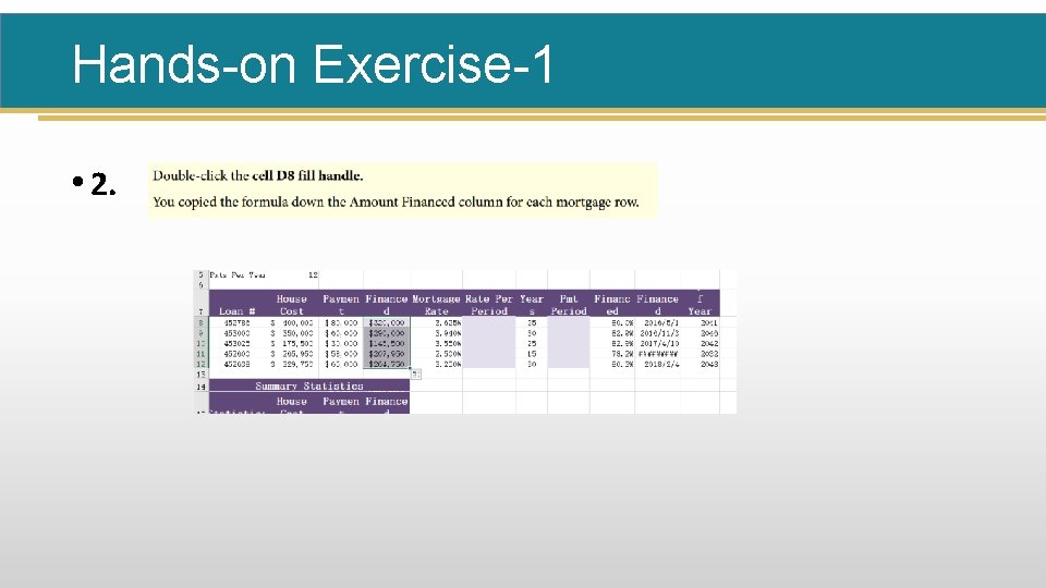
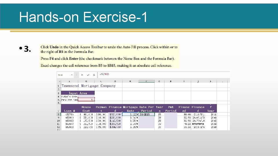
Hands-on Exercise-1 • Step 1: Use a relative cell reference in a formula • You need to calculate the amount financed by each borrower by creating a formula with relative cell references that calculates the difference between the house cost and the down payment. After verifying the results of the amount financed by the first borrower, you will copy the formula down the Amount Financed column to calculate the other borrowers’ amounts financed. Copyright © 2017 Pearson Education, Inc.

Hands-on Exercise-1 • 1.

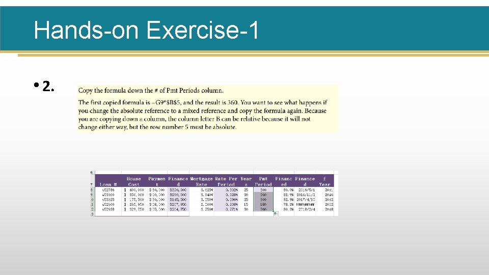
Hands-on Exercise-1 • 2.

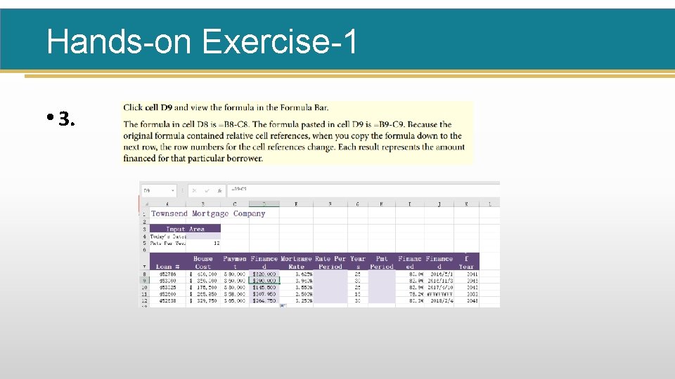
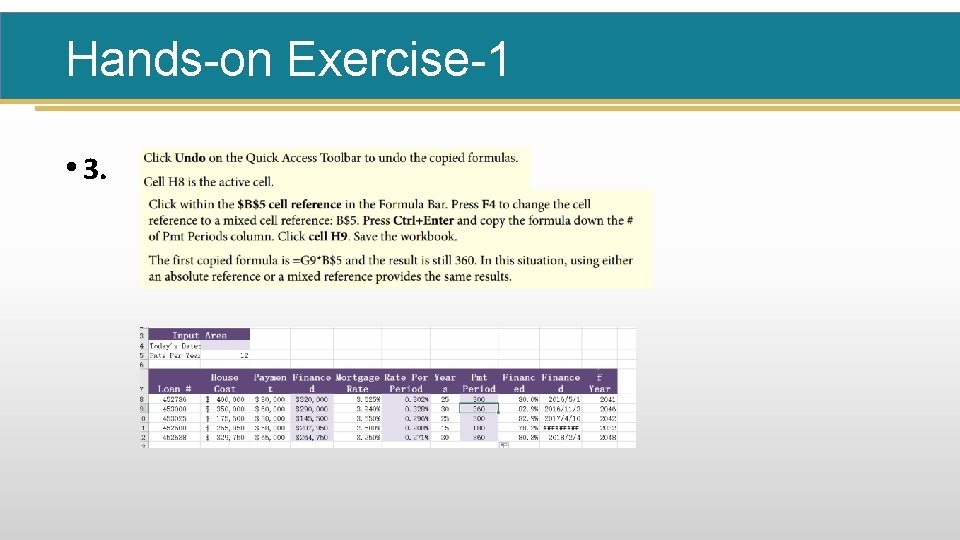
Hands-on Exercise-1 • 3.

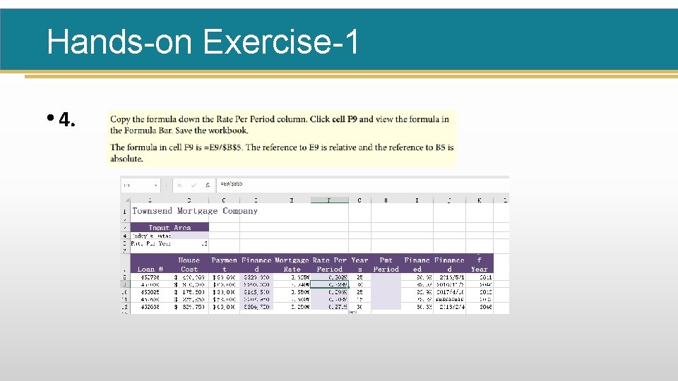
Hands-on Exercise-1 • Step 2: Use an absolute cell reference in a formula • Column E contains the annual percentage rate (APR) for each mortgage. Because the borrowers will make monthly payments, you need to calculate the monthly interest rate by dividing the APR by 12 (the number of payments in one year) for each borrower. Copyright © 2017 Pearson Education, Inc.

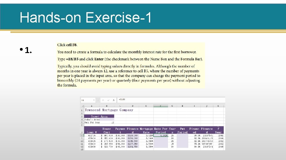
Hands-on Exercise-1 • 1.

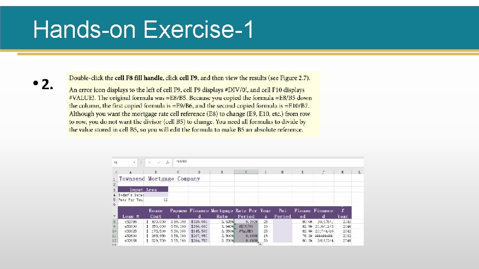
Hands-on Exercise-1 • 2.

Hands-on Exercise-1 • 3.

Hands-on Exercise-1 • 4.

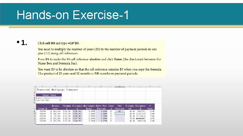
Hands-on Exercise-1 • Step 3: Use a mixed cell reference in a formula • The next formula you create will calculate the total number of payment periods for each loan. Copyright © 2017 Pearson Education, Inc.

Hands-on Exercise-1 • 1.

Hands-on Exercise-1 • 2.

Hands-on Exercise-1 • 3.

Objective 2: Insert a Function Skills: Insert a Function Using Formula Auto. Complete Use the Insert Function Dialog Box Copyright © 2017 Pearson Education, Inc.

Insert a Function • An Excel function is a predefined computation that simplifies creating a formula that performs a complex calculation. • When using functions, you must adhere to correct syntax, the rules that dictate the structure and components required to perform the necessary calculations. • Start a function with an equal sign, followed by the function name, and then its arguments in parentheses. Copyright © 2017 Pearson Education, Inc.

Insert a Function • Start a function with an equal sign, followed by the function name, and then its arguments in parentheses. • The function name describes the purpose of the function. For example, the function name SUM indicates that the function sums, or adds, values. • A function’s arguments specify the inputs—such as cells, values, or arithmetic expressions—that are required to complete the operation. In some cases, a function requires multiple arguments separated by commas. Copyright © 2017 Pearson Education, Inc.

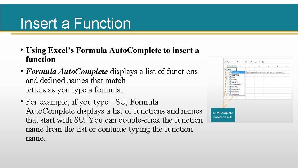
Insert a Function • Using Excel’s Formula Auto. Complete to insert a function • Formula Auto. Complete displays a list of functions and defined names that match letters as you type a formula. • For example, if you type =SU, Formula Auto. Complete displays a list of functions and names that start with SU. You can double-click the function name from the list or continue typing the function name.

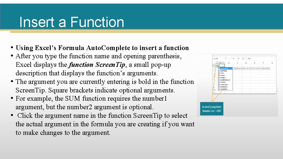
Insert a Function • Using Excel’s Formula Auto. Complete to insert a function • After you type the function name and opening parenthesis, Excel displays the function Screen. Tip, a small pop-up description that displays the function’s arguments. • The argument you are currently entering is bold in the function Screen. Tip. Square brackets indicate optional arguments. • For example, the SUM function requires the number 1 argument, but the number 2 argument is optional. • Click the argument name in the function Screen. Tip to select the actual argument in the formula you are creating if you want to make changes to the argument.

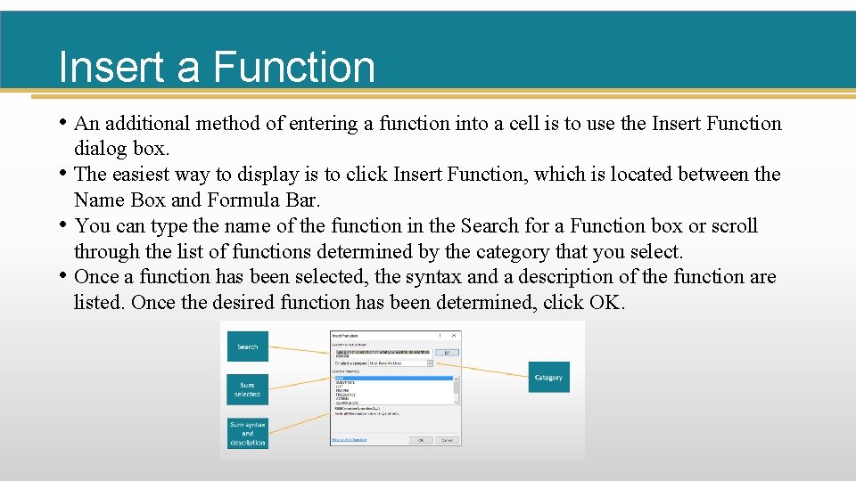
Insert a Function • An additional method of entering a function into a cell is to use the Insert Function dialog box. • The easiest way to display is to click Insert Function, which is located between the Name Box and Formula Bar. • You can type the name of the function in the Search for a Function box or scroll through the list of functions determined by the category that you select. • Once a function has been selected, the syntax and a description of the function are listed. Once the desired function has been determined, click OK.

Objective 3: Insert Basic Math and Statistics Functions Skills: Use the SUM Function Use the MIN and MAX Functions Copyright © 2017 Pearson Education, Inc.

Insert Basic Math and Statistics Functions • Excel includes commonly used math and statistical functions that you can use for a variety of calculations. • For example, you can insert functions to calculate the total amount you spend on dining out in a month. Copyright © 2017 Pearson Education, Inc.

Insert Basic Math and Statistics Functions • The SUM function totals values in one or more cells and displays the result in the cell containing the function. • =SUM(number 1, [number 2], …) § =SUM(A 1, A 2, A 5) • The MIN function analyzes the range of cells in its argument list and determines the lowest value. • =MIN(number 1, [number 2], …) § =MIN(A 1, B 10: C 25) Copyright © 2017 Pearson Education, Inc.

Objective 4: Use Date Functions Skills: Use the TODAY Function Use the NOW Function Copyright © 2017 Pearson Education, Inc.

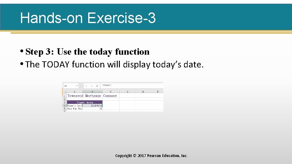
Use Date Functions • The TODAY function displays the current date in a cell. Excel updates the • • TODAY function each time the workbook is opened or printed. =TODAY() § Displays a result like: 2/9/2018 The NOW function uses the computer’s clock to display the current date and military time that the workbook was last opened. 14: 09 military time represents 2: 09 PM. =NOW() § Displays a result like: 2/9/2018 14: 09 Just note that these two functions do not require an argument. However, the empty parentheses are required. Copyright © 2017 Pearson Education, Inc.

Hands-on Exercise-2 • Download “e 02 h 1 Loans_Last. First ”, open it and save it as “e 02 hs. Loans_Last. First ”. • The Townsend Mortgage Company’s worksheet contains an area in which you must enter summary statistics. In addition, you need to include today’s date and identify the year in which each mortgage will be paid off. Copyright © 2017 Pearson Education, Inc.

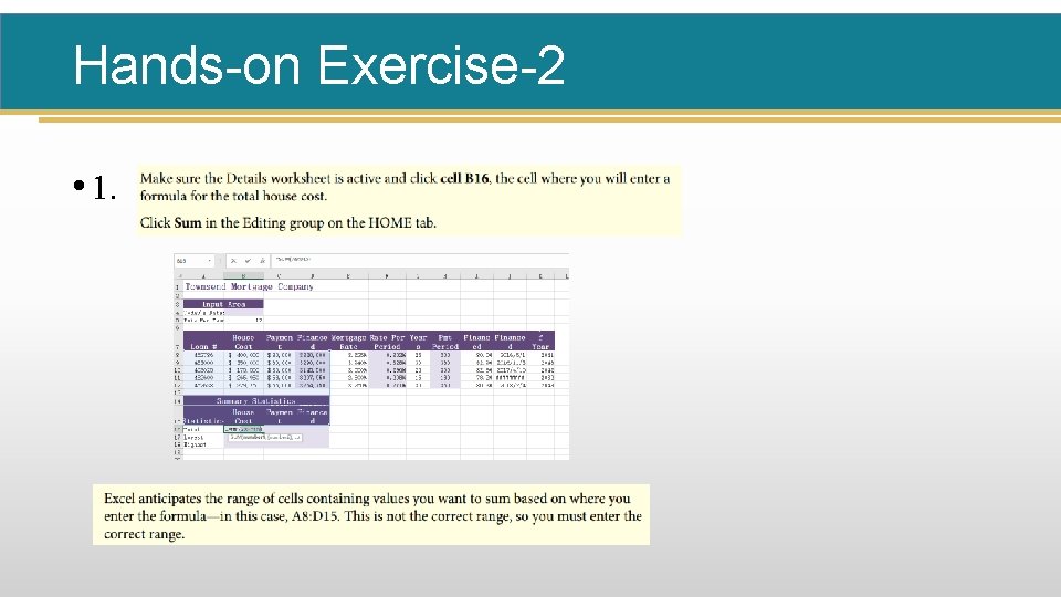
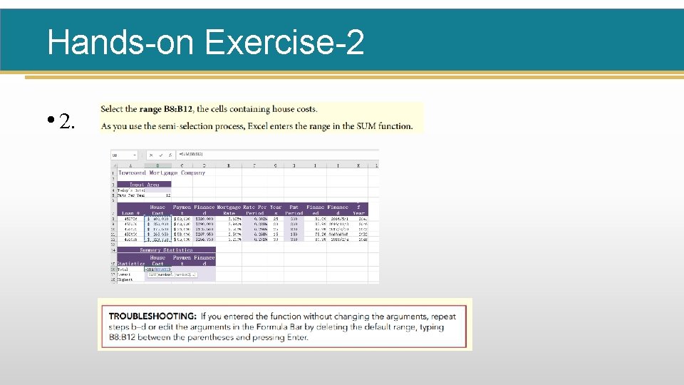
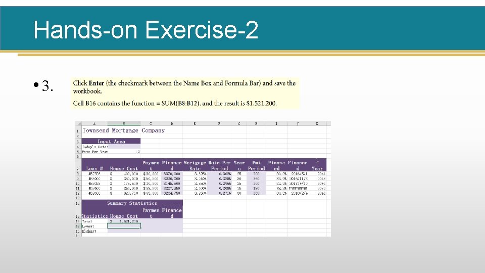
Hands-on Exercise-2 • Step 1: Use the sum function • The first summary statistic you need to calculate is the total value of the houses bought by the borrowers. You will use the SUM function. Copyright © 2017 Pearson Education, Inc.

Hands-on Exercise-2 • 1.

Hands-on Exercise-2 • 2.

Hands-on Exercise-2 • 3.

Hands-on Exercise-2 • Step 2: Use min and max functions • Erica wants to know the least and most expensive houses so that she can analyze typical customers of the Townsend Mortgage Company. You will use the MIN and MAX functions to obtain these statistics. Copyright © 2017 Pearson Education, Inc.

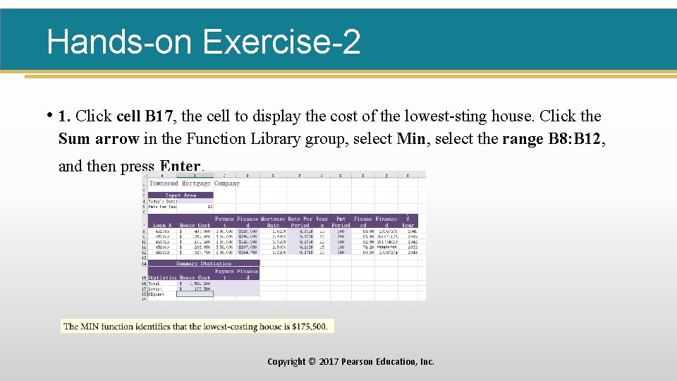
Hands-on Exercise-2 • 1. Click cell B 17, the cell to display the cost of the lowest-sting house. Click the Sum arrow in the Function Library group, select Min, select the range B 8: B 12, and then press Enter. Copyright © 2017 Pearson Education, Inc.

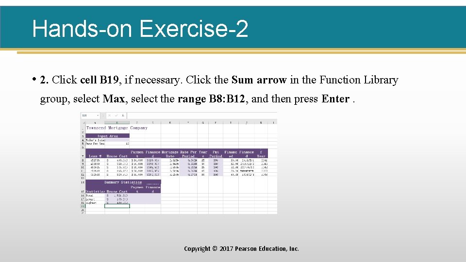
Hands-on Exercise-2 • 2. Click cell B 19, if necessary. Click the Sum arrow in the Function Library group, select Max, select the range B 8: B 12, and then press Enter. Copyright © 2017 Pearson Education, Inc.

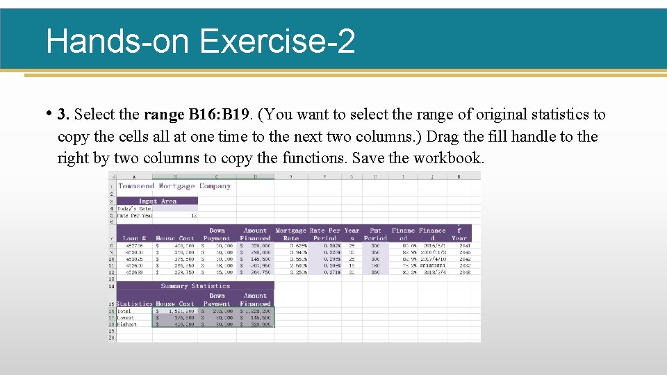
Hands-on Exercise-2 • 3. Select the range B 16: B 19. (You want to select the range of original statistics to copy the cells all at one time to the next two columns. ) Drag the fill handle to the right by two columns to copy the functions. Save the workbook.

Hands-on Exercise-3 • Step 3: Use the today function • The TODAY function will display today’s date. Copyright © 2017 Pearson Education, Inc.

Hands-on Exercise-3 • Step 3: Use the today function • The TODAY function will display today’s date. Copyright © 2017 Pearson Education, Inc.