Discrete Inference and Learning Lecture 4 Primaldual schema

Discrete Inference and Learning Lecture 4 Primal-dual schema, dual decomposition Yuliya Tarabalka yuliya. tarabalka@inria. fr Slides courtesy of Nikos Komodakis

Part I Recap: MRFs and Convex Relaxations

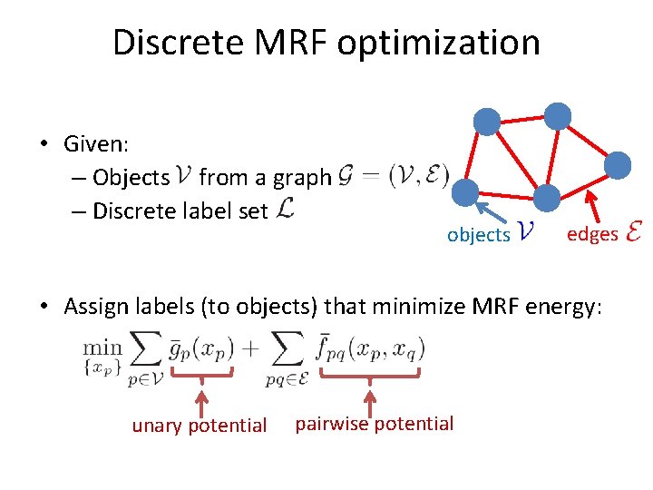
Discrete MRF optimization • Given: – Objects from a graph – Discrete label set objects edges • Assign labels (to objects) that minimize MRF energy: unary potential pairwise potential

Discrete MRF optimization • Extensive research for more than 20 years • MRF optimization ubiquitous in computer vision • segmentation optical flow image completion . . . stereo matching image restoration object detection/localization • and beyond • medical imaging, computer graphics, digital communications, physics… • Really powerful formulation

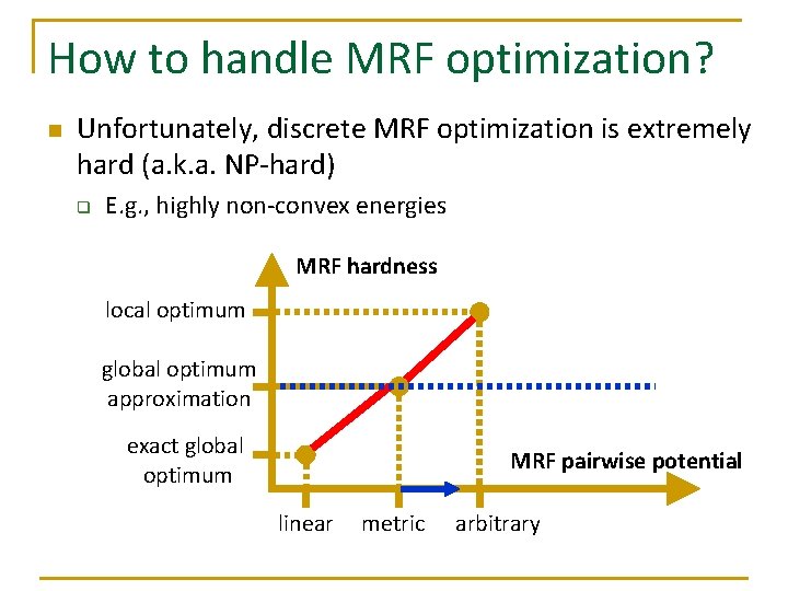
How to handle MRF optimization? n Unfortunately, discrete MRF optimization is extremely hard (a. k. a. NP-hard) q E. g. , highly non-convex energies MRF hardness local optimum global optimum approximation exact global optimum MRF pairwise potential linear metric arbitrary

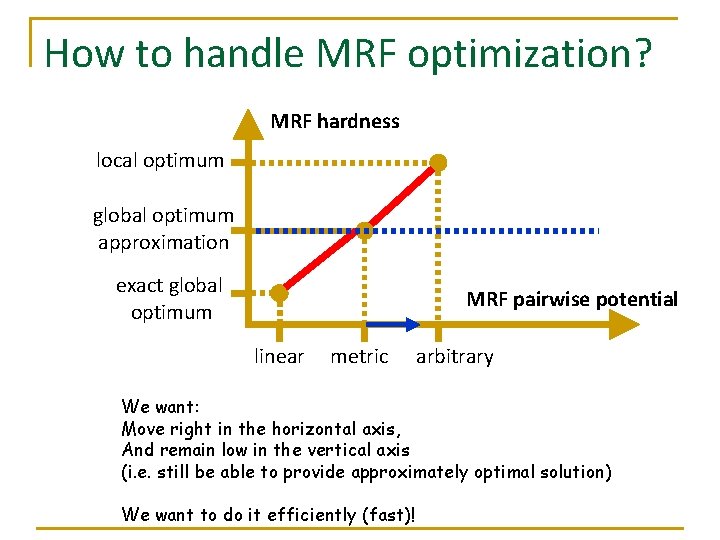
How to handle MRF optimization? MRF hardness local optimum global optimum approximation exact global optimum MRF pairwise potential linear metric arbitrary We want: Move right in the horizontal axis, And remain low in the vertical axis (i. e. still be able to provide approximately optimal solution) We want to do it efficiently (fast)!

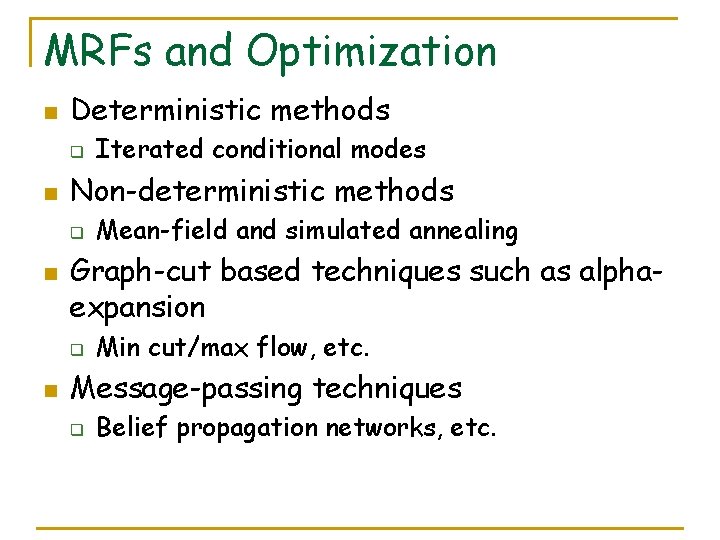
MRFs and Optimization n Deterministic methods q n Non-deterministic methods q n Mean-field and simulated annealing Graph-cut based techniques such as alphaexpansion q n Iterated conditional modes Min cut/max flow, etc. Message-passing techniques q Belief propagation networks, etc.

n n We would like to have a method which provides theoretical guarantees to obtain a good solution Within a reasonably fast computational time

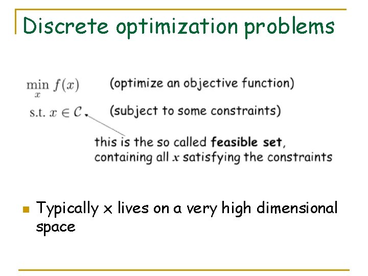
Discrete optimization problems n Typically x lives on a very high dimensional space

How to handle MRF optimization? n Unfortunately, discrete MRF optimization is extremely hard (a. k. a. NP-hard) q n So what do we do? q n n E. g. , highly non-convex energies Is there a principled way of dealing with this problem? Well, first of all, we don’t need to panic. Instead, we have to stay calm and RELAX! Actually, this idea of relaxing may not be such a bad idea after all…

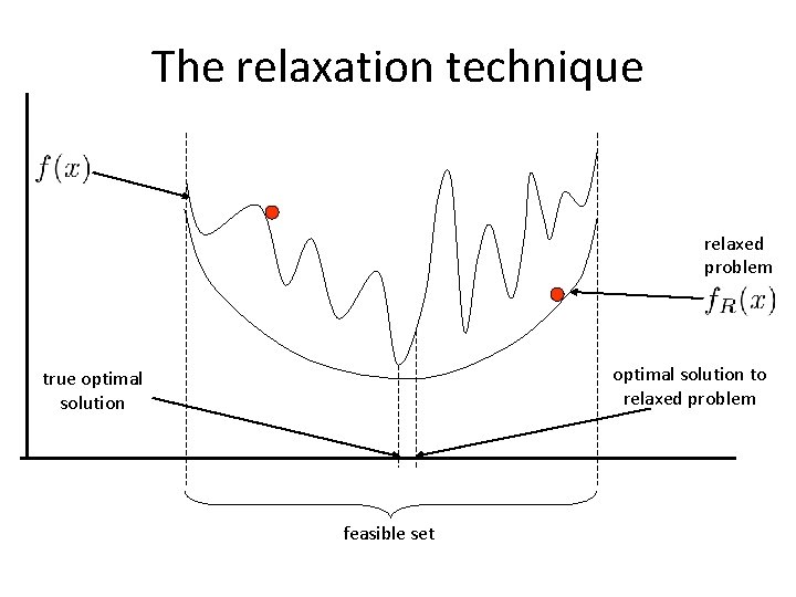
The relaxation technique n n Very successful technique for dealing with difficult optimization problems It is based on the following simple idea: q n try to approximate your original difficult problem with another one (the so called relaxed problem) which is easier to solve Practical assumptions: q q Relaxed problem must always be easier to solve Relaxed problem must be related to the original one

The relaxation technique relaxed problem optimal solution to relaxed problem true optimal solution feasible set

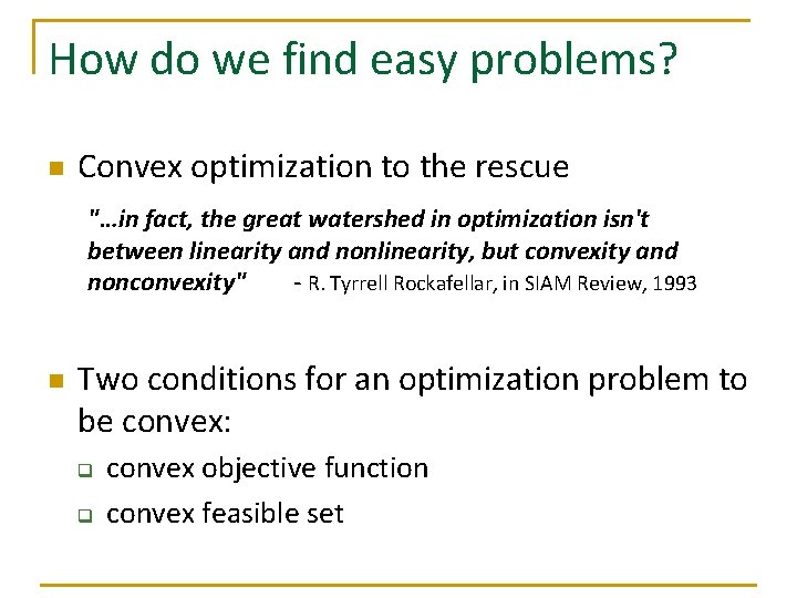
How do we find easy problems? n Convex optimization to the rescue "…in fact, the great watershed in optimization isn't between linearity and nonlinearity, but convexity and - R. Tyrrell Rockafellar, in SIAM Review, 1993 nonconvexity" n Two conditions for an optimization problem to be convex: q q convex objective function convex feasible set

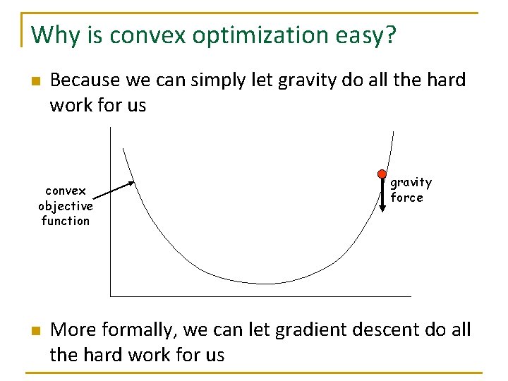
Why is convex optimization easy? n Because we can simply let gravity do all the hard work for us convex objective function n gravity force More formally, we can let gradient descent do all the hard work for us

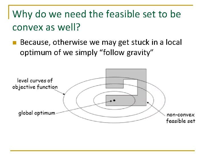
Why do we need the feasible set to be convex as well? n Because, otherwise we may get stuck in a local optimum of we simply “follow gravity”

How do we get a convex relaxation? n n n By dropping some constraints (so that the enlarged feasible set is convex) By modifying the objective function (so that the new function is convex) By combining both of the above

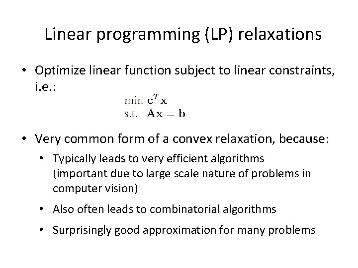
Linear programming (LP) relaxations • Optimize linear function subject to linear constraints, i. e. : • Very common form of a convex relaxation, because: • Typically leads to very efficient algorithms (important due to large scale nature of problems in computer vision) • Also often leads to combinatorial algorithms • Surprisingly good approximation for many problems

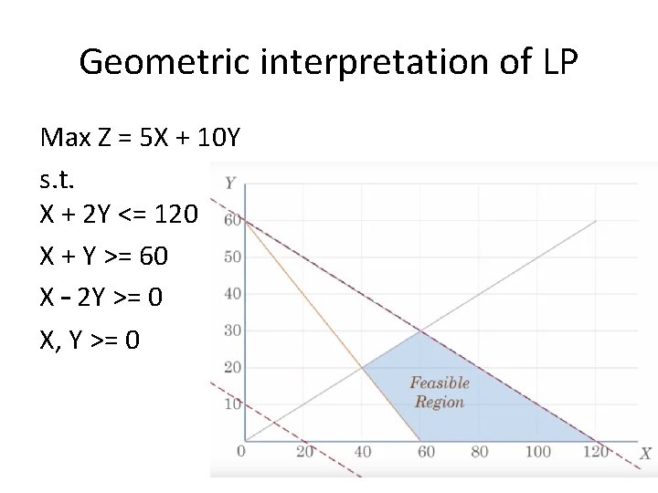
Geometric interpretation of LP Max Z = 5 X + 10 Y s. t. X + 2 Y <= 120 X + Y >= 60 X – 2 Y >= 0 X, Y >= 0

MRFs and Linear Programming • Tight connection between MRF optimization and Linear Programming (LP) recently emerged • Active research topic with a lot of interesting work: – MRFs and LP-relaxations [Schlesinger] [Boros] [Wainwright et al. 05] [Kolmogorov 05] [Weiss et al. 07] [Werner 07] [Globerson et al. 07] [Kohli et al. 08]… – Tighter/alternative relaxations [Sontag et al. 07, 08] [Werner 08] [Kumar et al. 07, 08]

MRFs and Linear Programming • E. g. , state of the art MRF algorithms are now known to be directly related to LP: – Graph-cut based techniques such as a-expansion: generalized by primal-dual schema algorithms (Komodakis et al. 05, 07) – Message-passing techniques: further generalized by Dual-Decomposition (Komodakis 07) • The above statement is more or less true for almost all state-of-the-art MRF techniques

Part II Primal-dual schema

The primal-dual schema n n Highly successful technique for exact algorithms. Yielded exact algorithms for cornerstone combinatorial problems: matching network flow minimum spanning tree minimum branching shortest path . . . Soon realized that it’s also an extremely powerful tool for deriving approximation algorithms [Vazirani]: set cover steiner network scheduling steiner tree feedback vertex set. . .

The primal-dual schema n Conjecture: Any approximation algorithm can be derived using the primal-dual schema (has not been disproved yet)

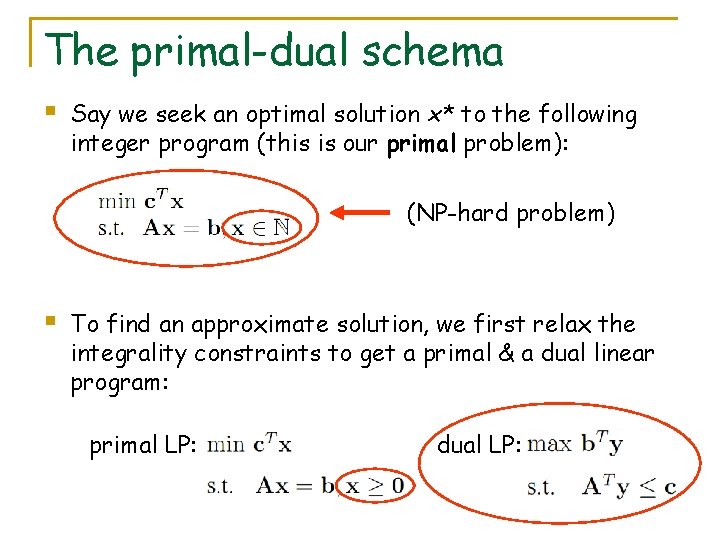
The primal-dual schema § Say we seek an optimal solution x* to the following integer program (this is our primal problem): (NP-hard problem) § To find an approximate solution, we first relax the integrality constraints to get a primal & a dual linear program: primal LP: dual LP:

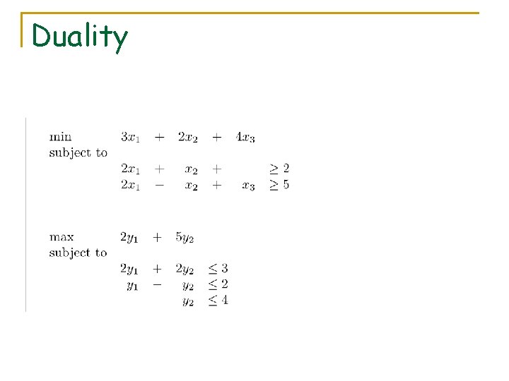
Duality

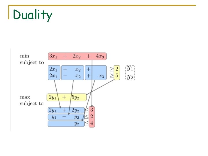
Duality

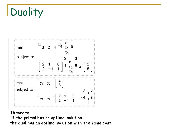
Duality Theorem: If the primal has an optimal solution, the dual has an optimal solution with the same cost

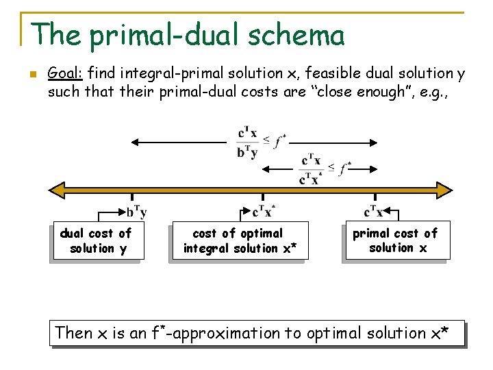
The primal-dual schema n Goal: find integral-primal solution x, feasible dual solution y such that their primal-dual costs are “close enough”, e. g. , dual cost of solution y cost of optimal integral solution x* primal cost of solution x Then x is an f*-approximation to optimal solution x*

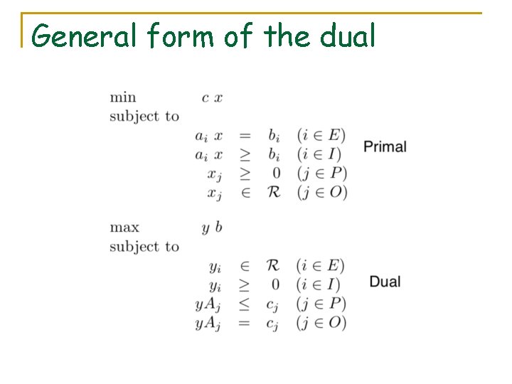
General form of the dual

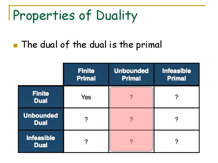
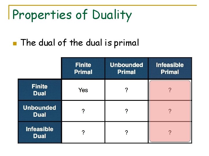
Properties of Duality n The dual of the dual is the primal

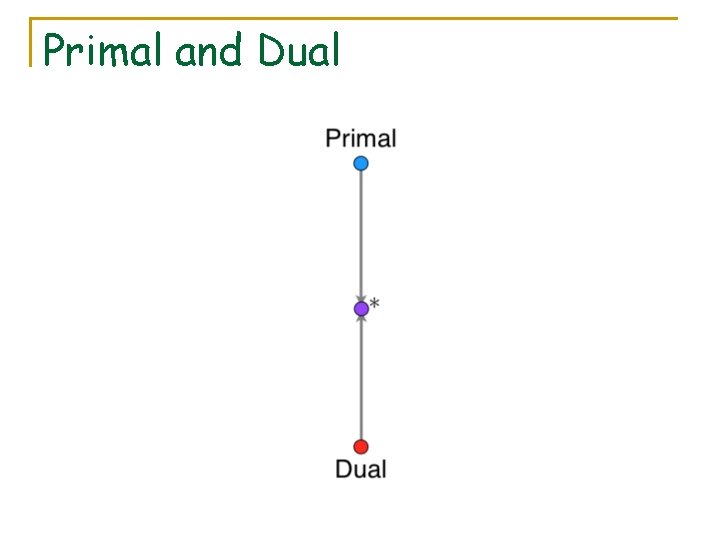
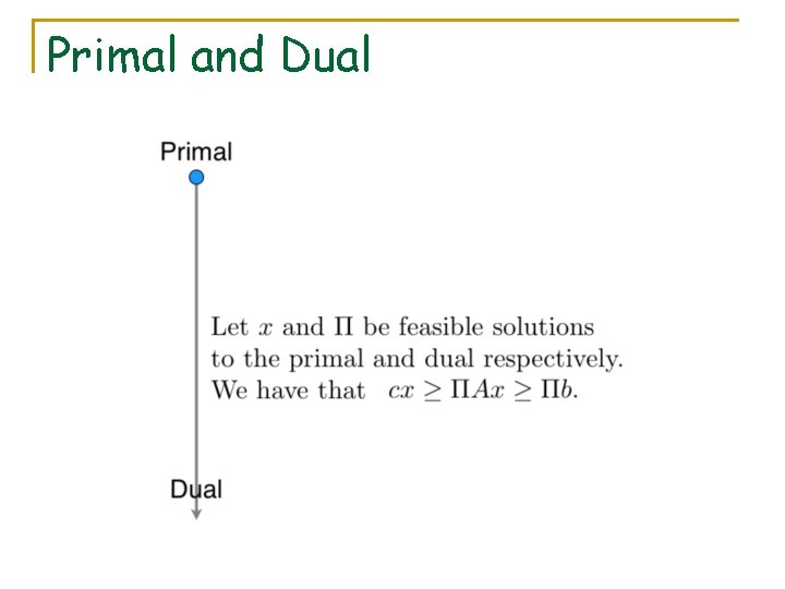
Primal and Dual

Properties of Duality n The dual of the dual is the primal

Primal and Dual

Properties of Duality n The dual of the dual is primal

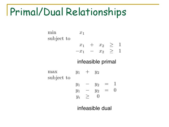
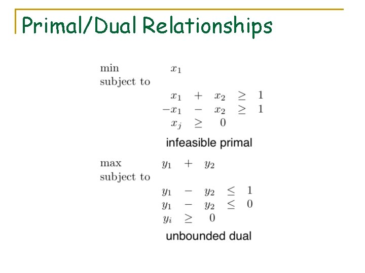
Primal/Dual Relationships

Primal/Dual Relationships

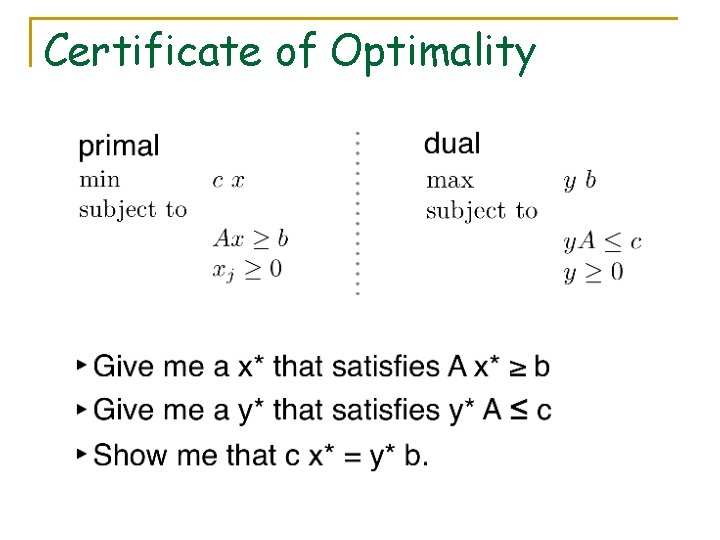
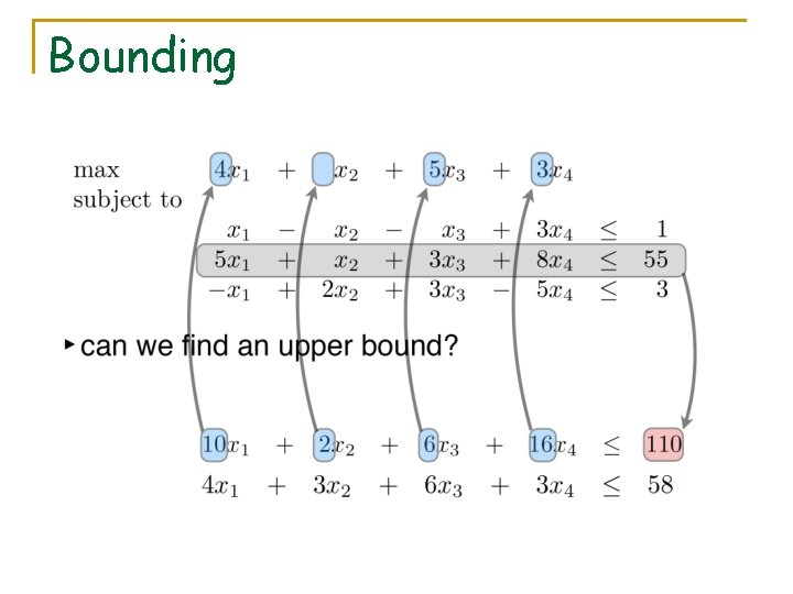
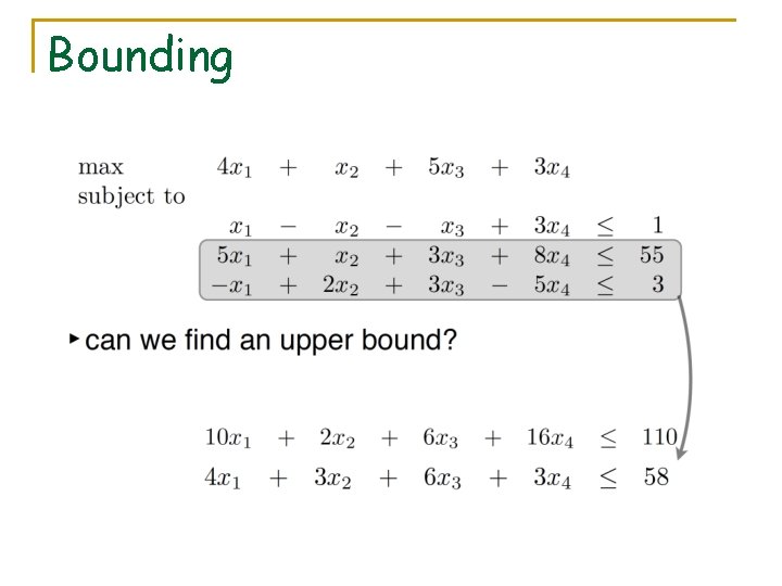
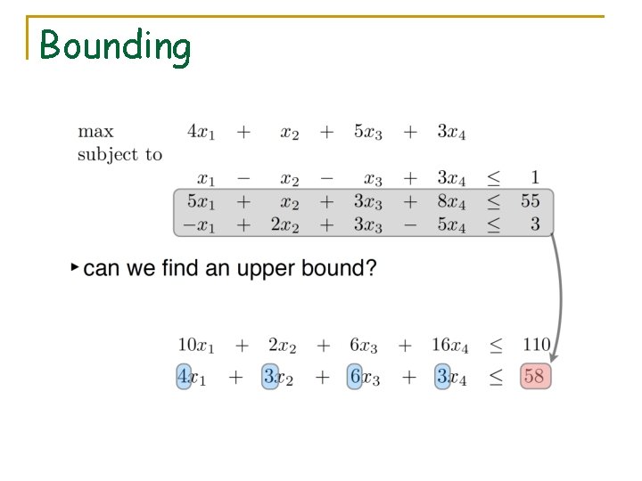
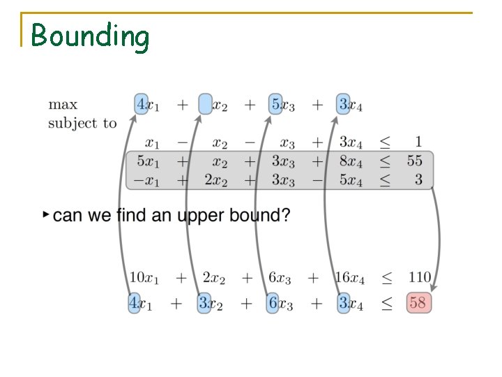
Certificate of Optimality n NP-complete problems q n Can you provide q n Certificate of feasibility A certificate of optimality? Consider now a linear program q Can you convince me that you have found an optimal solution?

Certificate of Optimality

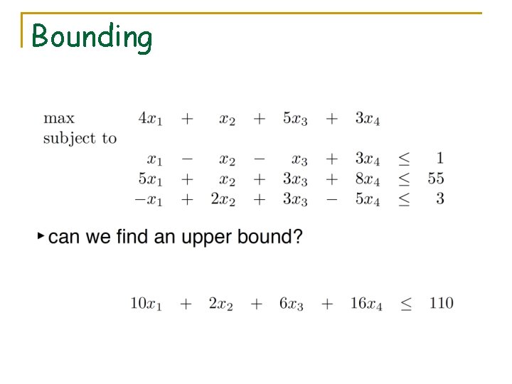
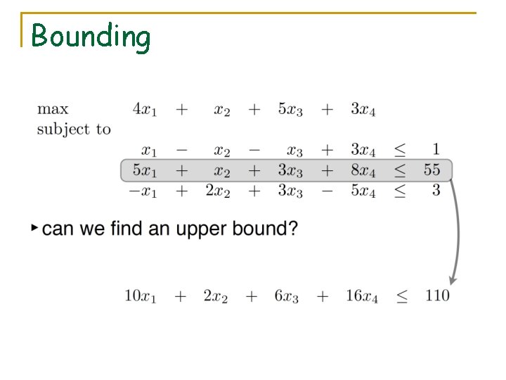
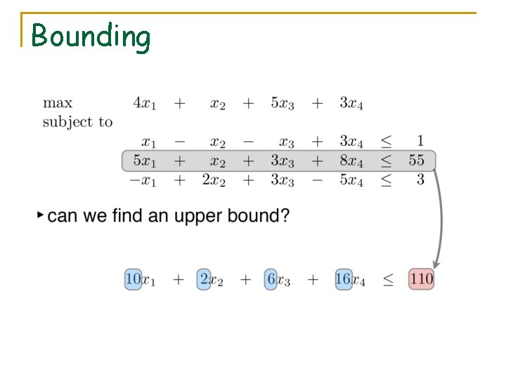
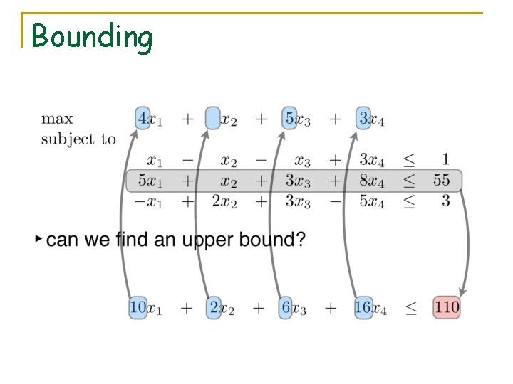
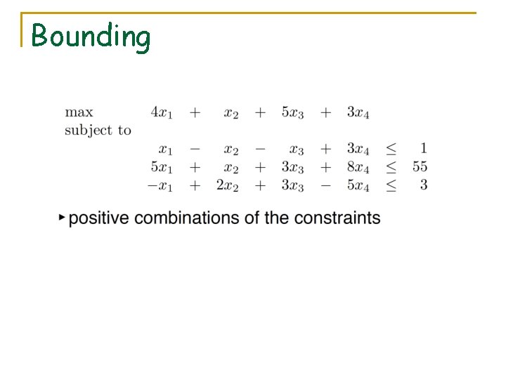
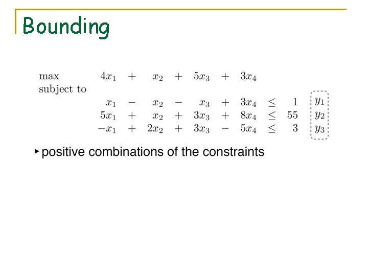
Bounding

Bounding

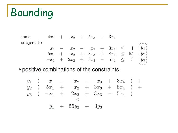
Bounding

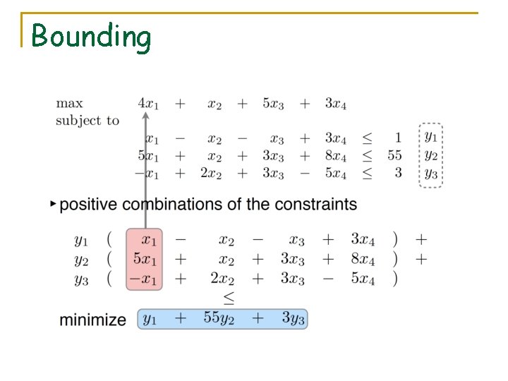
Bounding

Bounding

Bounding

Bounding

Bounding

Bounding

Bounding

Bounding

Bounding

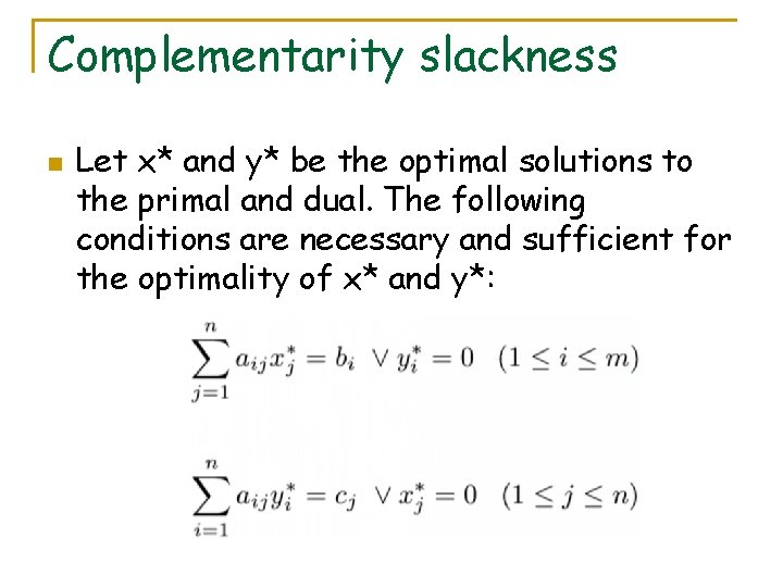
Complementarity slackness n Let x* and y* be the optimal solutions to the primal and dual. The following conditions are necessary and sufficient for the optimality of x* and y*:

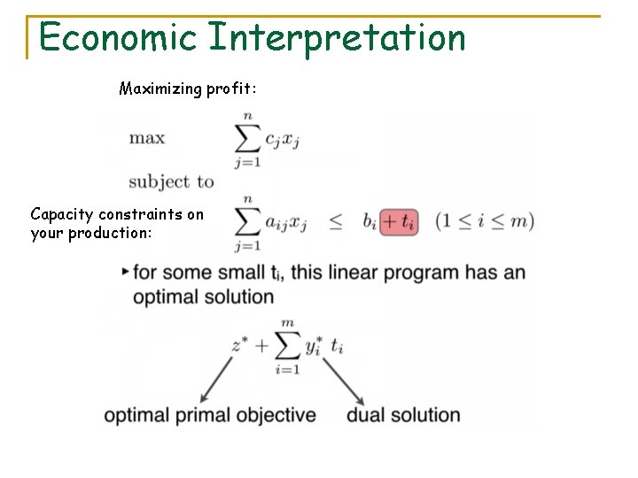
Economic Interpretation Maximizing profit: Capacity constraints on your production:

Primal-Dual n Why using the dual? q q q I have an optimal solution and I want to add a new constraint The dual is still feasible (I am adding a new variable); the primal is not Optimize the dual and the primal becomes feasible at optimality

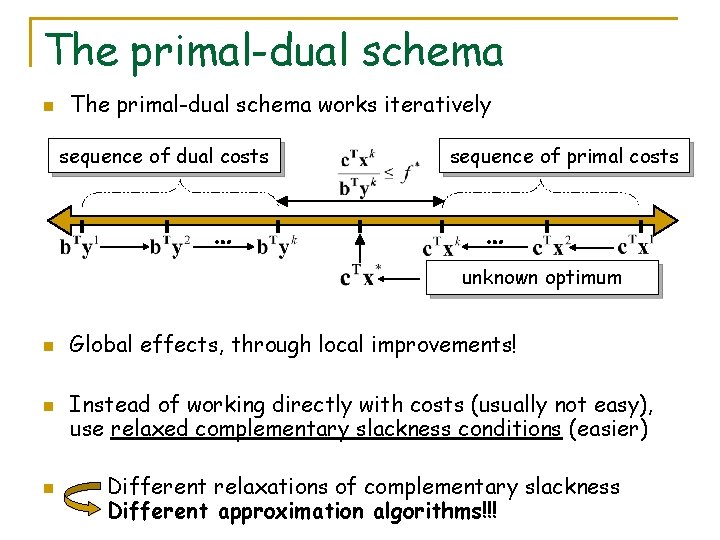
The primal-dual schema n The primal-dual schema works iteratively sequence of dual costs … sequence of primal costs … unknown optimum n n n Global effects, through local improvements! Instead of working directly with costs (usually not easy), use relaxed complementary slackness conditions (easier) Different relaxations of complementary slackness Different approximation algorithms!!!

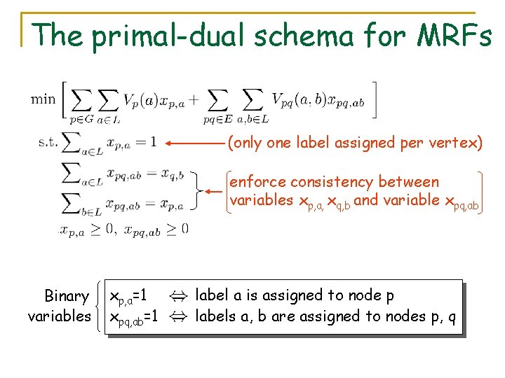
The primal-dual schema for MRFs (only one label assigned per vertex) enforce consistency between variables xp, a, xq, b and variable xpq, ab Binary variables xp, a=1 xpq, ab=1 label a is assigned to node p labels a, b are assigned to nodes p, q

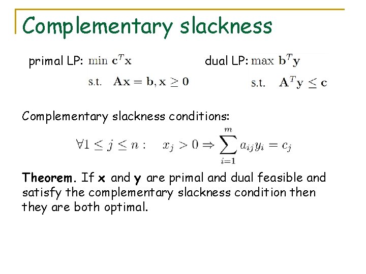
Complementary slackness primal LP: dual LP: Complementary slackness conditions: Theorem. If x and y are primal and dual feasible and satisfy the complementary slackness condition they are both optimal.

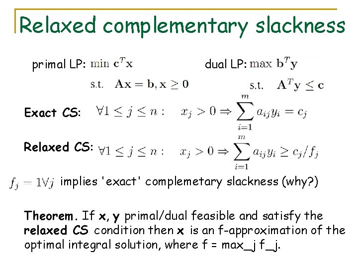
Relaxed complementary slackness primal LP: dual LP: Exact CS: Relaxed CS: implies 'exact' complemetary slackness (why? ) Theorem. If x, y primal/dual feasible and satisfy the relaxed CS condition then x is an f-approximation of the optimal integral solution, where f = max_j f_j.

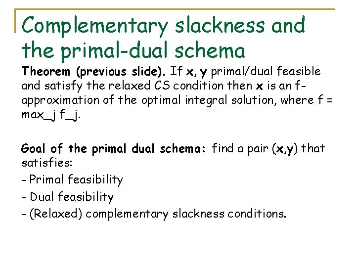
Complementary slackness and the primal-dual schema Theorem (previous slide). If x, y primal/dual feasible and satisfy the relaxed CS condition then x is an fapproximation of the optimal integral solution, where f = max_j f_j. Goal of the primal dual schema: find a pair (x, y) that satisfies: - Primal feasibility - Dual feasibility - (Relaxed) complementary slackness conditions.

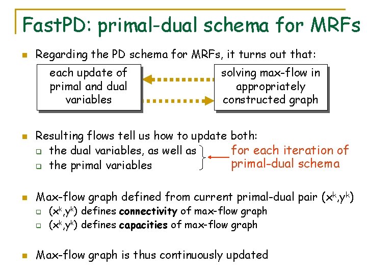
Fast. PD: primal-dual schema for MRFs n Regarding the PD schema for MRFs, it turns out that: each update of primal and dual variables n n Resulting flows tell us how to update both: for each iteration of q the dual variables, as well as primal-dual schema q the primal variables Max-flow graph defined from current primal-dual pair (x k, yk) q q n solving max-flow in appropriately constructed graph (xk, yk) defines connectivity of max-flow graph (xk, yk) defines capacities of max-flow graph Max-flow graph is thus continuously updated

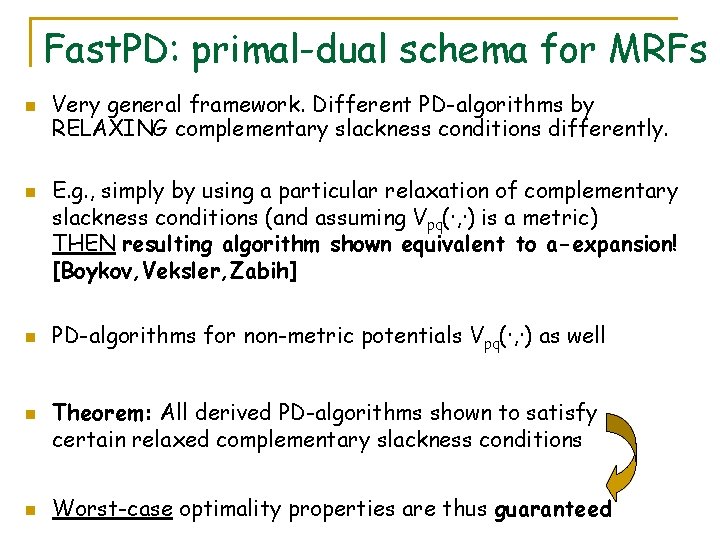
Fast. PD: primal-dual schema for MRFs n n n Very general framework. Different PD-algorithms by RELAXING complementary slackness conditions differently. E. g. , simply by using a particular relaxation of complementary slackness conditions (and assuming Vpq(·, ·) is a metric) THEN resulting algorithm shown equivalent to a-expansion! [Boykov, Veksler, Zabih] PD-algorithms for non-metric potentials Vpq(·, ·) as well Theorem: All derived PD-algorithms shown to satisfy certain relaxed complementary slackness conditions Worst-case optimality properties are thus guaranteed

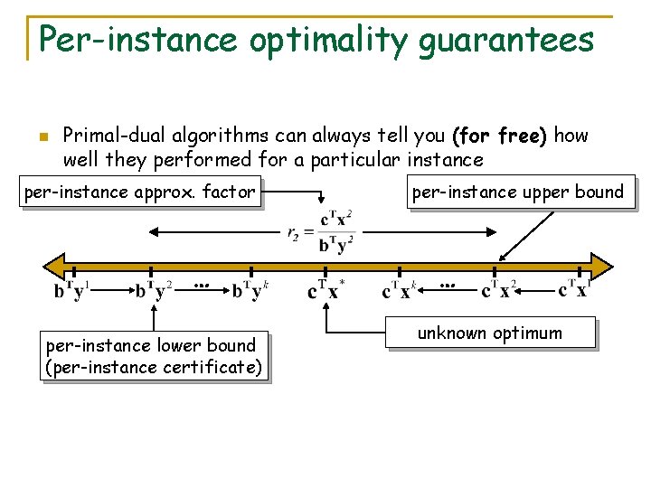
Per-instance optimality guarantees n Primal-dual algorithms can always tell you (for free) how well they performed for a particular instance per-instance approx. factor … per-instance lower bound (per-instance certificate) per-instance upper bound … unknown optimum

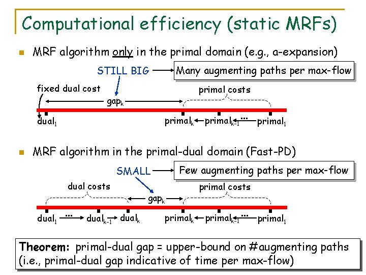
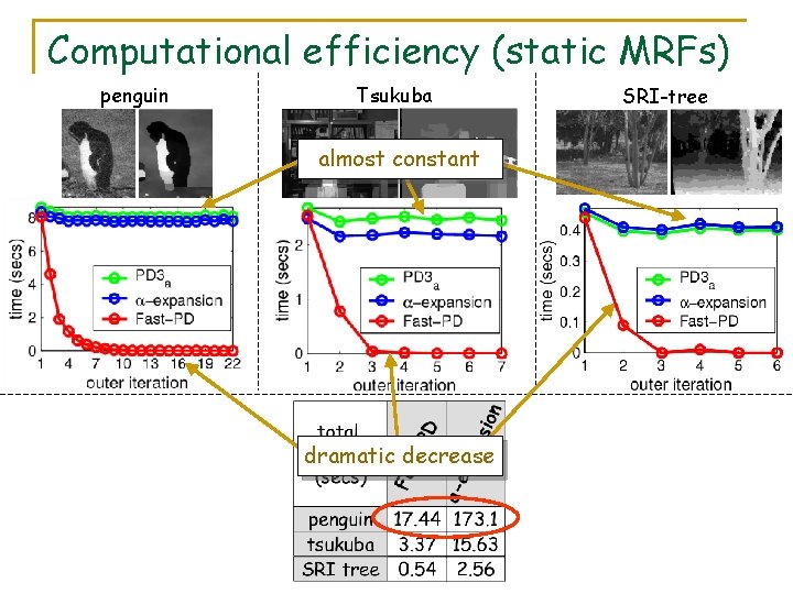
Computational efficiency (static MRFs) n MRF algorithm only in the primal domain (e. g. , a-expansion) Many augmenting paths per max-flow STILL BIG fixed dual cost primal costs gapk primalk dual 1 n primalk-1 … primal 1 MRF algorithm in the primal-dual domain (Fast-PD) Few augmenting paths per max-flow SMALL dual costs dual 1 … dualk-1 dualk gapk primal costs primalk-1 … primal 1 Theorem: primal-dual gap = upper-bound on #augmenting paths (i. e. , primal-dual gap indicative of time per max-flow)

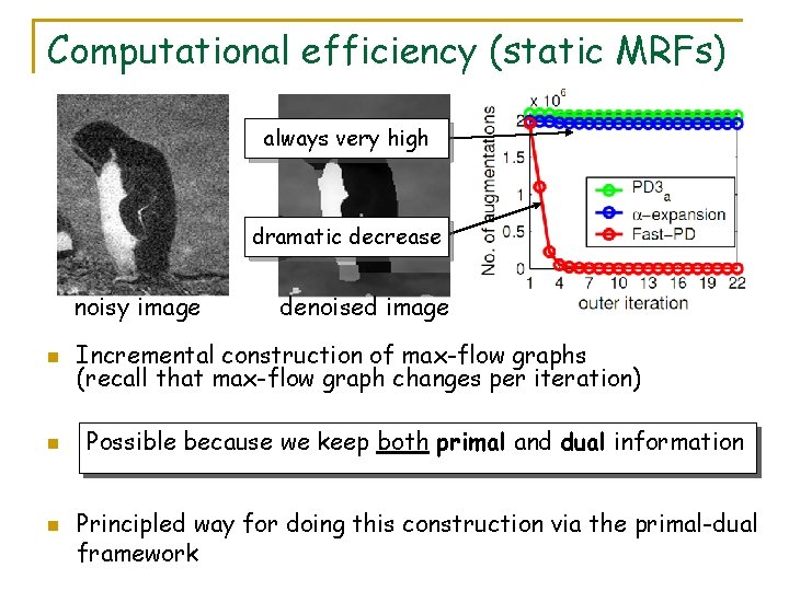
Computational efficiency (static MRFs) always very high dramatic decrease noisy image n n n denoised image Incremental construction of max-flow graphs (recall that max-flow graph changes per iteration) Possible because we keep both primal and dual information Principled way for doing this construction via the primal-dual framework

Computational efficiency (static MRFs) penguin Tsukuba almost constant dramatic decrease SRI-tree

Computational efficiency (dynamic MRFs) n Fast-PD can speed up dynamic MRFs [Kohli, Torr] as well (demonstrates the power and generality of this framework) gap dualy SMALL primalx few path augmentations Fast-PD algorithm SMALL gap primalx dual 1 fixed dual cost n LARGE SMALL many path augmentations primal-based algorithm Principled (and simple) way to update dual variables when switching between different MRFs

Drop: Deformable Registration using Discrete Optimization [Glocker et al. 07, 08] n n n Easy to use GUI Main focus on medical imaging 2 D-2 D registration 3 D-3 D registration Publicly available: http: //campar. in. tum. de/Main/Drop

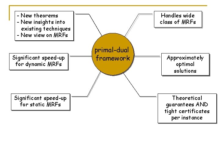
- New theorems - New insights into existing techniques - New view on MRFs Significant speed-up for dynamic MRFs Significant speed-up for static MRFs Handles wide class of MRFs primal-dual framework Approximately optimal solutions Theoretical guarantees AND tight certificates per instance

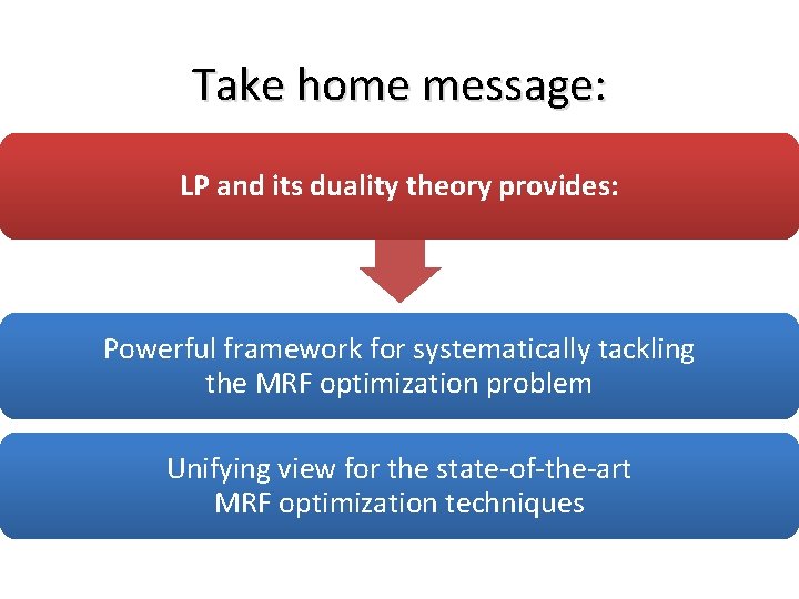
Take home message: LP and its duality theory provides: Powerful framework for systematically tackling the MRF optimization problem Unifying view for the state-of-the-art MRF optimization techniques