Differential Analysis of Fluid Flow Part II Potential


 in the x direction; (b) in arbitrary direction Uniform")
 in the x direction; (b) in arbitrary direction Uniform")


 Sink –")
 Sink –")


")


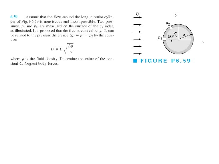
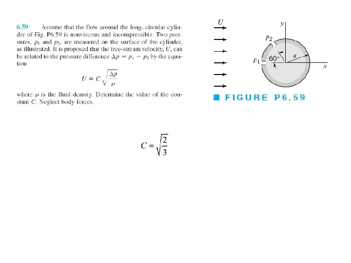
 developed on the cylinder can be determined")
 developed on the cylinder can be determined")

")


 Consider equal strength, source-sink pair. combined stream function for the pair is")
 Put (b) and (c) into (a) then For small values of a")
 Let source and sink approach one another (a 0) while increasing the")


- Slides: 78
Differential Analysis of Fluid Flow Part II Potential Flows
Irrotational Flow Analysis of inviscid flow can be simplified by an assumption of irrotational flow. For irrotational flow vorticity is zero: Condition of irrotationality imposes specific relationship among velocity gradients. Since Then
Uniform Flow
Examples Flow fields involving real fluids often include both regions of negligible shearing stresses and regions of significant shearing stresses Uniform flow in x direction Various regions of flow: (a) around bodies; (b) through channels
Bernoulli Equation for Irrotational Flow Start from For irrotational flow Thus, Bernoulli equation Between any two points in the flow field. Now, Bernoulli equation is restricted to inviscid, steady, incompressible, irrotational flow
Velocity Potential For irrotational flow velocity components can be expressed in term of scalar function (x, y, z, t)
Velocity Potential For irrotational flow velocity components can be expressed in term of scalar function (x, y, z, t) where is called the velocity potential (distinguish from stream function). In vector form
Velocity Potential For irrotational flow velocity components can be expressed in term of scalar function (x, y, z, t) where is called the velocity potential (distinguish from stream function). In vector form For incompressible, irrotational flow Inviscid, incompressible, irrotational flow fields are governed by Laplace’s equation and are called potential flows In cylindrical polar coordinates, velocity components Laplace’s equation
Example 6. 4: The two-dimensional flow of a nonviscous, incompressible fluid in the vicinity of the 90º corner is described by the stream function where has units of m 2/s when r is in meters. (a) Determine, if possible, the corresponding velocity potential. (b) If the pressure at point (1) on the wall is 30 k. Pa, what is the pressure at point (2)? Assume the fluid density is 103 kg/m 3 and the x–y plane is horizontal, that is, there is no difference in elevation between points (1) and (2)
Example 6. 4: The two-dimensional flow of a nonviscous, incompressible fluid in the vicinity of the 90º corner is described by the stream function where has units of m 2/s when r is in meters. (a) Determine, if possible, the corresponding velocity potential. (b) If the pressure at point (1) on the wall is 30 k. Pa, what is the pressure at point (2)? Assume the fluid density is 103 kg/m 3 and the x–y plane is horizontal, that is, there is no difference in elevation between points (1) and (2) Solution: (a) Velocity components Velocity potential
Example 6. 4: The two-dimensional flow of a nonviscous, incompressible fluid in the vicinity of the 90º corner is described by the stream function where has units of m 2/s when r is in meters. (a) Determine, if possible, the corresponding velocity potential. (b) If the pressure at point (1) on the wall is 30 k. Pa, what is the pressure at point (2)? Assume the fluid density is 103 kg/m 3 and the x–y plane is horizontal, that is, there is no difference in elevation between points (1) and (2) Solution: (b) Apply Bernoulli equation between (1) and (2)
Example 6. 4: The two-dimensional flow of a nonviscous, incompressible fluid in the vicinity of the 90º corner is described by the stream function where has units of m 2/s when r is in meters. (a) Determine, if possible, the corresponding velocity potential. (b) If the pressure at point (1) on the wall is 30 k. Pa, what is the pressure at point (2)? Assume the fluid density is 103 kg/m 3 and the x–y plane is horizontal, that is, there is no difference in elevation between points (1) and (2) Solution: (b) Apply Bernoulli equation between (1) and (2)
Basic, Plane Potential Flows
Basic, Plane Potential Flows • Laplace’s equation is a linear partial differential equation • For potential flow, basic solutions can be added to obtain more complicated solutions • Only plane flows will be considered • For plane irrotational flow one can use either velocity potential or the stream function – both must satisfy Laplace’s equation • Flow net consists of a family of streamlines and equipotential lines
Uniform Flow Uniform flow: (a) in the x direction; (b) in arbitrary direction Uniform flow can be described by either a stream function of a velocity potential.
Uniform Flow Uniform flow: (a) in the x direction; (b) in arbitrary direction Uniform flow can be described by either a stream function of a velocity potential. For case (a) for case (b)
Source and Sink Consider fluid flowing radially outward from a line through the origin perpendicular to x-y plane Let m be the volume flow rate of flow emanating from the line (per unit length).
Source and Sink Consider fluid flowing radially outward from a line through the origin perpendicular to x-y plane Let m be the volume flow rate of flow emanating from the line (per unit length). To satisfy conservation mass Since the flow is a purely radial, Velocity potential Stream function
Source and Sink Source – m is positive (flow is radyally outward) Sink – m is negative, (flow is toward the origin) m is called the strength of the source (sink) A source or sink represent a purely radial flow
Source and Sink Source – m is positive (flow is radyally outward) Sink – m is negative, (flow is toward the origin) m is called the strength of the source (sink) A source or sink represent a purely radial flow At the origin r = 0 and which is impossible Thus, sources and sinks do not really exist in real flow fields, and the line representing the source or sink is a mathematical singularity in the flow field. However, some real flows can be approximated at points away from the origin by using sources of sinks
Example 6. 5 Nonviscous, incompressible fluid flows between wedge-shaped walls into a small opening. Velocity potential (in ft 2/s), which approximately describes this flow is Determine the volume rate of flow (per unit length) into the opening
Example 6. 5 Nonviscous, incompressible fluid flows between wedge-shaped walls into a small opening. Velocity potential (in ft 2/s), which approximately describes this flow is Determine the volume rate of flow (per unit length) into the opening Solution Velocity components Flowrate Note that the radius R is arbitrary since the flowrate crossing any curve between the two walls must be the same. The negative sign indicate that the flow is toward the opening
Vortex Consider a flow field in which the streamlines are concentric circles, that is interchange the velocity potential and stream function for the source where K is a constant
Vortex Consider a flow field in which the streamlines are concentric circles, that is interchange the velocity potential and stream function for the source where K is a constant In this case streamlines are concentric circles with Vortex represents a flow in which the streamlines are concentric circles Tangential velocity varies inversely with the distance from the origin, with a singularity occurring at r = 0 Vortex motion can be either rotational or irrotational
Free Vortex • • • Is vortex irrotational flow? Rotation refers to the orientation of fluid element and not the path followed by the element Free vortex is a potential flow Irrotational (free) vortex Rotational (forced) vortex
Forced Vortex • • If fluid rotates as a rigid body, vortex flow is rotational (forced vortex) Forced vortex is not potential flow Irrotational (free) vortex Rotational (forced) vortex
Combined Vortex Combined vortex is one with a forced vortex as a central core and a velocity distribution corresponding to that of a free vortex outside the core. For a combined vortex where K and are constants and r 0 corresponds to the radius of the central core Irrotational (free) vortex Rotational (forced) vortex
Circulation , , is the line integral of the tangential component of the velocity taken around a closed curve in the flow field
Circulation , , is the line integral of the tangential component of the velocity taken around a closed curve in the flow field For irrotational flow
Circulation If there are singularities enclosed within the curve circulation may not be zero. For free vortex: Velocity potential and stream function for the free vortex are commonly expressed in terms of the circulation as
Example 6. 6 A liquid drains from a large tank through a small opening. A vortex forms whose velocity distribution away from the tank opining can be approximated as that of a free vortex having a velocity potential Determine an expression relating the surface shape to the strength of the vortex as specified by the circulation
Example 6. 6 A liquid drains from a large tank through a small opening. A vortex forms whose velocity distribution away from the tank opining can be approximated as that of a free vortex having a velocity potential Determine an expression relating the surface shape to the strength of the vortex as specified by the circulation Solution Apply Bernoulli equation between (1) and (2) Velocity Expression for surface shape
Doublet is formed by a source and sink approach one another (a → 0) (details) K is a strength of the doublet
Doublet Streamlines for a doublet are circles through the origin tangent to the x axis.
Summary of Basic Potential Flows
Superposition of Basic, Plane Potential Flows
Superposition of Basic, Plane Potential Flows • Potential flows are governed by Laplace’s equation, which is linear partial differential equation. • Various basic velocity potentials and stream functions can be combined to form new potentials and stream functions. • Any streamline in an inviscid flow field can be considered as a solid boundary (no flow through the boundary or the streamline) • If we combine some basic velocity potentials or stream functions to yield a streamline that corresponds to a particular body shape, that combination can be used to describe the flow around that body. • This method is called the method of superposition
Source in a Uniform Stream – Half-Body Flow around a half-body is obtained by the addition of a source to a uniform flow Stream function and velocity potential:
Source in a Uniform Stream – Half-Body Flow around a half-body is obtained by the addition of a source to a uniform flow Stream function and velocity potential Stagnation point will occur at
Source in a Uniform Stream – Half-Body Flow around a half-body is obtained by the addition of a source to a uniform flow Stream function and velocity potential Stagnation point will occur at x = -b (r = b ), where
Source in a Uniform Stream – Half-Body Value of stream function at stagnation point (r = b and = ) Equation of the streamline passing through stagnation point
Source in a Uniform Stream – Half-Body Value of stream function at stagnation point (r = b and = ) Equation of the streamline passing through stagnation point
Source in a Uniform Stream – Half-Body Replace streamline passing through stagnation point with solid boundary and get the flow around streamlined body placed in uniform stream. The body is open at downstream end, and is called a half-body. Singularity (source) occurs inside the body, and there are no singularity in the flow field of interest (outside the body) Width of the half-body asymptotically approaches 2 b (details)
Source in a Uniform Stream – Half-Body Velocity for half-body
Source in a Uniform Stream – Half-Body For half-body Square of magnitude of velocity, V, at any point and since With velocity known, the pressure at any point can be determined from Bernoulli equation
Example 6. 7 The shape of a hill arising from a plain can be approximated with the top section of a halfbody as is illustrated in Figure. The height of the hill approaches 200 ft as shown. (a) When a 40 mi/hr wind blows toward the hill, what is the magnitude of the air velocity at a point on the hill directly above the origin [point (2)]? (b) What is the elevation of point (2) above the plain and what is the difference in pressure between point (1) on the plain far from the hill and point (2)? Assume an air density of 0. 00238 slugs/ft 3
Example 6. 7 The shape of a hill arising from a plain can be approximated with the top section of a halfbody as is illustrated in Figure. The height of the hill approaches 200 ft as shown. (a) When a 40 mi/hr wind blows toward the hill, what is the magnitude of the air velocity at a point on the hill directly above the origin [point (2)]? (b) What is the elevation of point (2) above the plain and what is the difference in pressure between point (1) on the plain far from the hill and point (2)? Assume an air density of 0. 00238 slugs/ft 3 Solution (a) Velocity:
Example 6. 7 The shape of a hill arising from a plain can be approximated with the top section of a halfbody as is illustrated in Figure. The height of the hill approaches 200 ft as shown. (a) When a 40 mi/hr wind blows toward the hill, what is the magnitude of the air velocity at a point on the hill directly above the origin [point (2)]? (b) What is the elevation of point (2) above the plain and what is the difference in pressure between point (1) on the plain far from the hill and point (2)? Assume an air density of 0. 00238 slugs/ft 3 Solution (a) Velocity: At point (2), = /2, and Thus
Example 6. 7 The shape of a hill arising from a plain can be approximated with the top section of a halfbody as is illustrated in Figure. The height of the hill approaches 200 ft as shown. (a) When a 40 mi/hr wind blows toward the hill, what is the magnitude of the air velocity at a point on the hill directly above the origin [point (2)]? (b) What is the elevation of point (2) above the plain and what is the difference in pressure between point (1) on the plain far from the hill and point (2)? Assume an air density of 0. 00238 slugs/ft 3 Solution (b) Elevation of point (2)
Example 6. 7 The shape of a hill arising from a plain can be approximated with the top section of a halfbody as is illustrated in Figure. The height of the hill approaches 200 ft as shown. (a) When a 40 mi/hr wind blows toward the hill, what is the magnitude of the air velocity at a point on the hill directly above the origin [point (2)]? (b) What is the elevation of point (2) above the plain and what is the difference in pressure between point (1) on the plain far from the hill and point (2)? Assume an air density of 0. 00238 slugs/ft 3 Solution (b) Elevation of point (2) From Bernoulli equation
Rankine Ovals Rankine ovals are formed b combining a source and sink with a uniform flow. alternatively Flow around a Rankine oval: (a) superposition of source-sink pair and a uniform flow; (b) replacement of streamline = 0 with solid boundary to form Rankine oval
Rankine Ovals Streamline with = 0 forms closed body which is called Rankine oval Flow around a Rankine oval: (a) superposition of source-sink pair and a uniform flow; (b) replacement of streamline = 0 with solid boundary to form Rankine oval
Rankine Ovals Stagnation points occur at the upstream and downstream ends of the body Location of stagnation points depend on a, m and U Flow around a Rankine oval: (a) superposition of source-sink pair and a uniform flow; (b) replacement of streamline = 0 with solid boundary to form Rankine oval
Rankine Ovals Body half-width, h, equals value of y where y axis intersect = 0 streamline Flow around a Rankine oval: (a) superposition of source-sink pair and a uniform flow; (b) replacement of streamline = 0 with solid boundary to form Rankine oval
Rankine Ovals Parameter Ua/m determines body shape Large value of Ua/m – flow around long slender body Small value of Ua/m – flow around blunt body Flow around a Rankine oval: (a) superposition of source-sink pair and a uniform flow; (b) replacement of streamline = 0 with solid boundary to form Rankine oval
Doublet combined with a uniform flow can be used to represent flow around a circular cylinder. Stream function, velocity potential and velocity components: (details) Flow Around of Circular Cylinder
Doublet combined with a uniform flow can be used to represent flow around a circular cylinder. Stream function, velocity potential and velocity components: (details) On the surface of the cylinder (r = a) Flow Around of Circular Cylinder
Doublet combined with a uniform flow can be used to represent flow around a circular cylinder. Stream function, velocity potential and velocity components: (details) On the surface of the cylinder (r = a) Maximum velocity, 2 U, occurs at the top and bottom of the cylinder and reduces to U far away from cylinder as we move along the ray = /2 Flow Around of Circular Cylinder
Pressure distribution on the cylinder surface is obtained from Bernoulli equation Pressure Distribution
Pressure distribution on the cylinder surface is obtained from Bernoulli equation Only on the upstream part of the cylinder is there approximate agreement between the potential flow and the experimental results Because to the viscous boundary layer that develops on the cylinder, the main flow separates from the surface of the cylinder, leading to the large difference between theoretical, frictionless fluid solution ant the experimental results on the downstream side of the cylinder Pressure Distribution
d’Alembert Paradox Resultant force (per unit length) developed on the cylinder can be determined by integrating the pressure over the surface. Drag (force parallel to direction of the uniform flow)
d’Alembert Paradox Resultant force (per unit length) developed on the cylinder can be determined by integrating the pressure over the surface. Drag (force parallel to direction of the uniform flow) Lift (force perpendicular to direction of the uniform flow) Substitution for ps and integration gives Fx = 0 and Fy = 0 Thus, drag and lift as predicted by potential theory for a fixed cylinder in a uniform flow are zero However, we know from experience that there is a significant drag developed on a cylinder when it is placed in a moving fluid This discrepancy is known as d’Alembert paradox
Flow Around Rotating Cylinder Flow around the rotating cylinder is obtained by adding free vortex to flow around a cylinder. Stream function and velocity potential: Tangential velocity on the surface of the cylinder (r = a) Variety of streamline patterns can be developed, depending on the vortex strength Location of stagnation point is obtained from expression
Flow Around Rotating Cylinder The location of stagnation points on a circular cylinder: (a) without circulation; (b, c, d) with circulation.
Magnus Effect For cylinder with circulation: surface pressure drag lift Thus, fro the cylinder with circulation lift is developed If U is positive (in the positive x direction) and is positive (free vortex with counterclockwise rotation) lift is downward Development of lift on rotating bodies is called the Magnus effect
End of lecture
Supplementary Slides
Tell Apart Stream Function Velocity Potential Consequence of conservation of mass Consequence of irrotationality Restricted to twodimensional flow Can be defined for threedimensional flow back
For plane irrotational flow In cylindrical coordinates For irrotational flow and in terms of stream function or back
Flow net for a 90º bend back
Lines of constant are streamlines, that is Change in Along line of constant we have so that Flow net for a 90º bend back
Doublet (derivation) Consider equal strength, source-sink pair. combined stream function for the pair is
Doublet (derivation) Put (b) and (c) into (a) then For small values of a
Doublet (derivation) Let source and sink approach one another (a 0) while increasing the strength m (m ) so that the product ma/ remains constant. In this case r/(r 2 – a 2) 1/r and where K is the strength of the doublet back
back
Doublet combined with a uniform flow can be used to represent flow around a circular cylinder Flow Around of Circular Cylinder To represent flow around circular cylinder stream function must be constant for r = a, where a is the radius of the cylinder. From it follows that = 0 for r = a if Thus stream function and velocity potential for flow around circular cylinder are back