CSC 211 Data Structures Lecture 16 Dr Iftikhar

CSC 211 Data Structures Lecture 16 Dr. Iftikhar Azim Niaz ianiaz@comsats. edu. pk 1

Last Lecture Summary n n Complexity of Bubble Sort Selection Sort q q n n Complexity of Selection Sort Insertion Sort q q n Concept and Algorithm Code and Implementation Complexity of Insertion Sort 2

Objectives Overview n Comparison of Sorting methods q q q n Bubble, Selection and Insertion Recursion q q q Concept Example Implementation Code 3

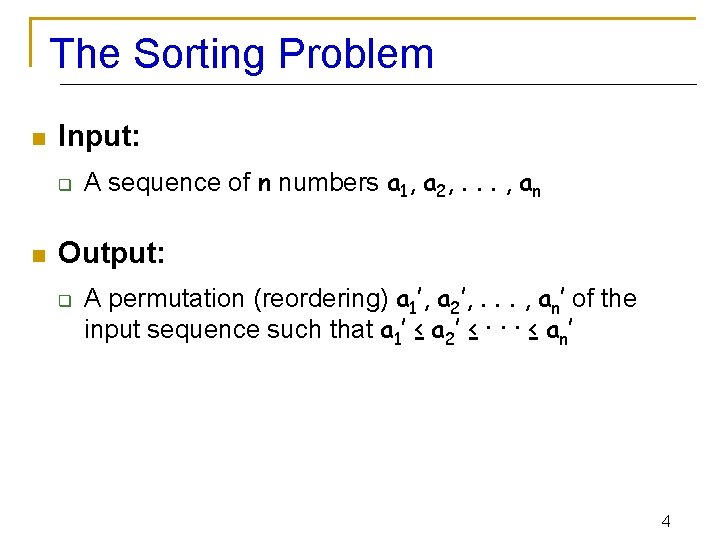
The Sorting Problem n Input: q n A sequence of n numbers a 1, a 2, . . . , an Output: q A permutation (reordering) a 1’, a 2’, . . . , an’ of the input sequence such that a 1’ ≤ a 2’ ≤ · · · ≤ an’ 4

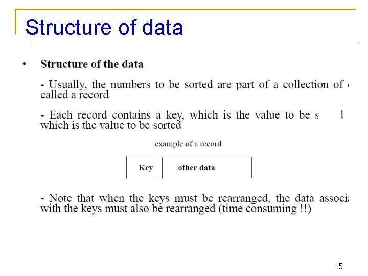
Structure of data 5

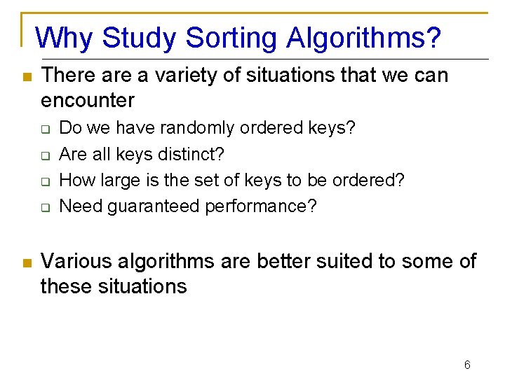
Why Study Sorting Algorithms? n There a variety of situations that we can encounter q q n Do we have randomly ordered keys? Are all keys distinct? How large is the set of keys to be ordered? Need guaranteed performance? Various algorithms are better suited to some of these situations 6

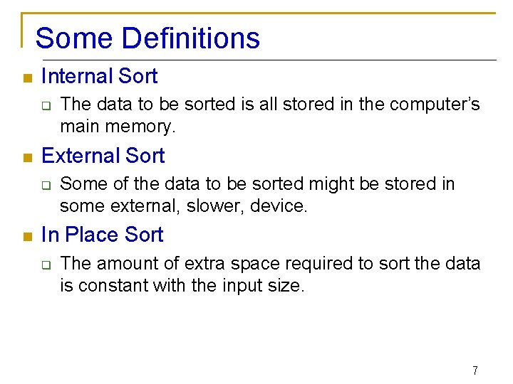
Some Definitions n Internal Sort q n External Sort q n The data to be sorted is all stored in the computer’s main memory. Some of the data to be sorted might be stored in some external, slower, device. In Place Sort q The amount of extra space required to sort the data is constant with the input size. 7

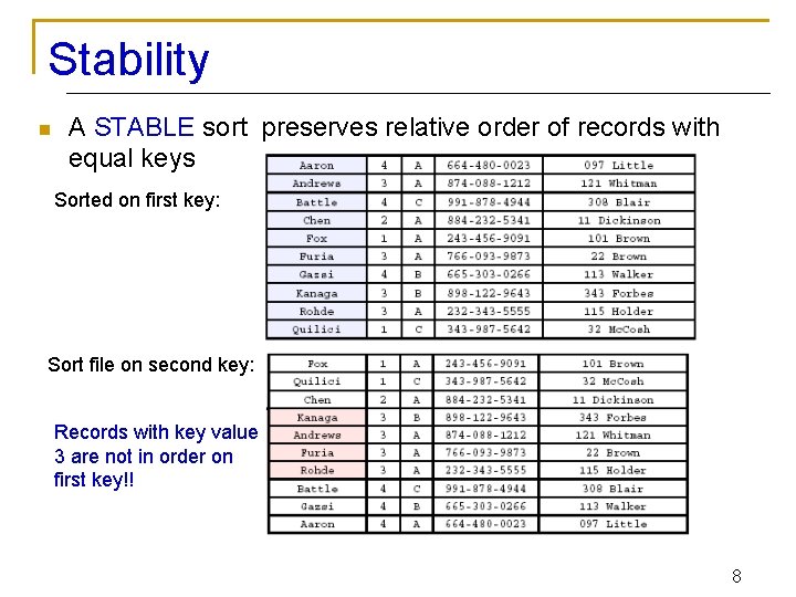
Stability n A STABLE sort preserves relative order of records with equal keys Sorted on first key: Sort file on second key: Records with key value 3 are not in order on first key!! 8

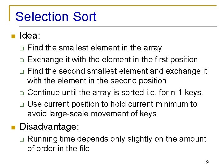
Selection Sort n Idea: q q q n Find the smallest element in the array Exchange it with the element in the first position Find the second smallest element and exchange it with the element in the second position Continue until the array is sorted i. e. for n-1 keys. Use current position to hold current minimum to avoid large-scale movement of keys. Disadvantage: q Running time depends only slightly on the amount of order in the file 9

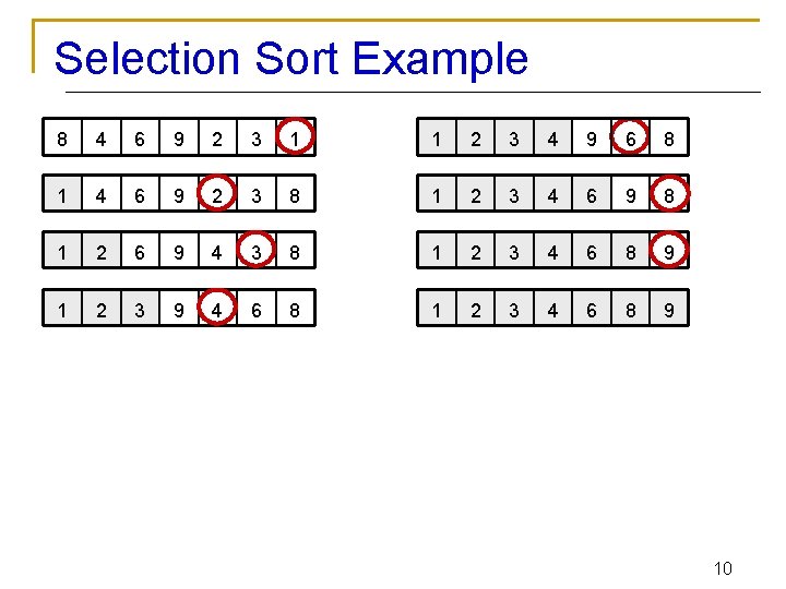
Selection Sort Example 8 4 6 9 2 3 1 1 2 3 4 9 6 8 1 4 6 9 2 3 8 1 2 3 4 6 9 8 1 2 6 9 4 3 8 1 2 3 4 6 8 9 1 2 3 9 4 6 8 1 2 3 4 6 8 9 10

Selection Sort Alg. : SELECTION-SORT(A) n ← length[A] 8 4 6 9 for j ← 1 to n - 1 do smallest ← j for i ← j + 1 to n do if A[i] < A[smallest] then smallest ← i exchange A[j] ↔ A[smallest] 2 3 1 11

Selection Sort: Analysis Alg. : SELECTION-SORT(A) n ← length[A] Fixed n-1 iterations for j ← 1 to n - 1 n 2/2 do smallest ← j comparisonsfor n exchanges cost c 1 1 c 2 n Fixed n-i iterations c 3 i ← j + 1 to n c 4 do if A[i] < A[smallest] c 5 then smallest ← i times n-1 c 6 exchange A[j] ↔ A[smallest] c 7 n-1 12

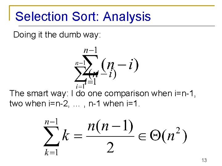
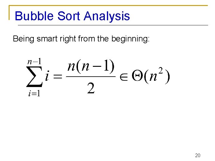
Selection Sort: Analysis Doing it the dumb way: The smart way: I do one comparison when i=n-1, two when i=n-2, … , n-1 when i=1. 13

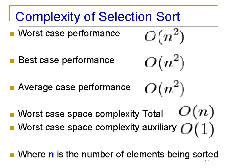
Complexity of Selection Sort n Worst case performance n Best case performance n Average case performance n n Worst case space complexity Total Worst case space complexity auxiliary n Where n is the number of elements being sorted 14

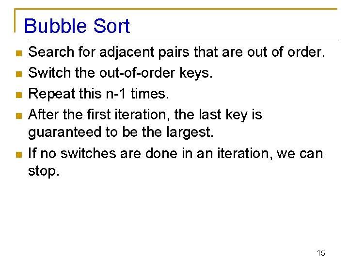
Bubble Sort n n n Search for adjacent pairs that are out of order. Switch the out-of-order keys. Repeat this n-1 times. After the first iteration, the last key is guaranteed to be the largest. If no switches are done in an iteration, we can stop. 15

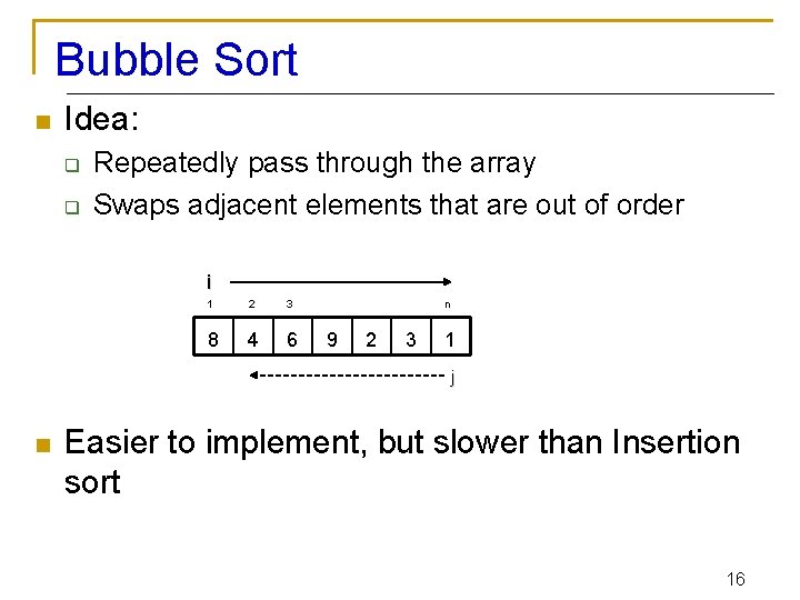
Bubble Sort n Idea: q q Repeatedly pass through the array Swaps adjacent elements that are out of order i 1 2 3 8 4 6 n 9 2 3 1 j n Easier to implement, but slower than Insertion sort 16

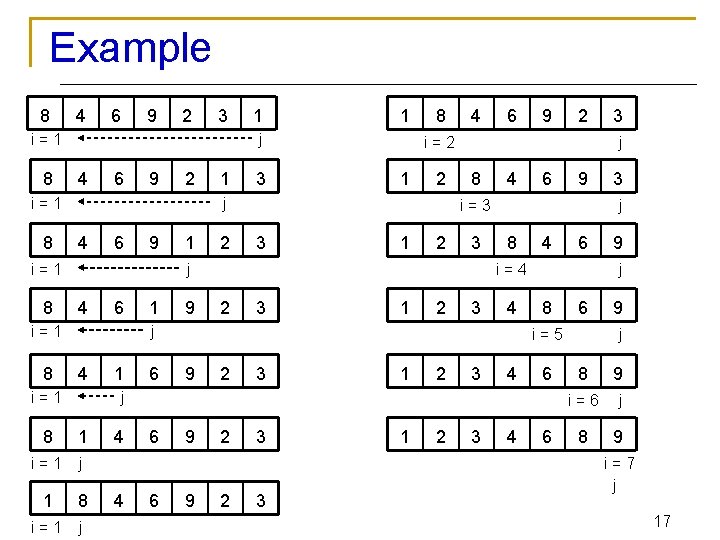
Example 8 4 6 9 2 3 i=1 8 4 6 9 2 4 6 3 9 1 2 4 4 6 1 9 6 i=1 1 6 1 2 8 4 6 1 i=1 j 1 8 i=1 j 4 4 6 6 9 i=3 3 1 2 3 8 4 6 i=4 2 3 1 2 3 9 9 2 2 3 3 1 2 3 3 4 4 4 9 j 8 6 i=5 9 3 j 6 j 8 2 j j 4 9 i=2 j i=1 8 1 6 9 j 8 9 i=6 j 8 9 i=7 j 17

Bubble Sort Alg. : BUBBLESORT(A) for i 1 to length[A] do for j length[A] downto i + 1 do if A[j] < A[j -1] then exchange A[j] A[j-1] i 8 i=1 4 6 9 2 3 1 j 18

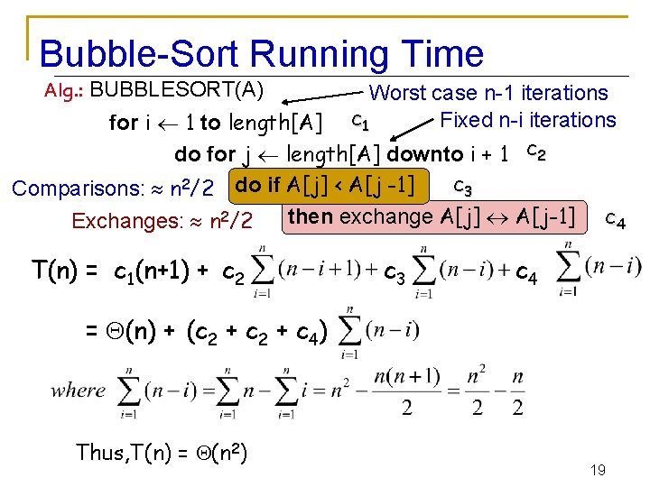
Bubble-Sort Running Time Alg. : BUBBLESORT(A) Worst case n-1 iterations Fixed n-i iterations for i 1 to length[A] c 1 do for j length[A] downto i + 1 c 2 c 3 Comparisons: n 2/2 do if A[j] < A[j -1] then exchange A[j] A[j-1] Exchanges: n 2/2 T(n) = c 1(n+1) + c 2 c 3 c 4 = (n) + (c 2 + c 4) Thus, T(n) = (n 2) 19

Bubble Sort Analysis Being smart right from the beginning: 20

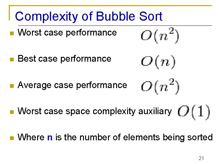
Complexity of Bubble Sort n Worst case performance n Best case performance n Average case performance n Worst case space complexity auxiliary n Where n is the number of elements being sorted 21

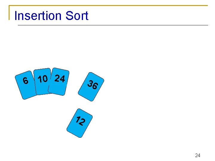
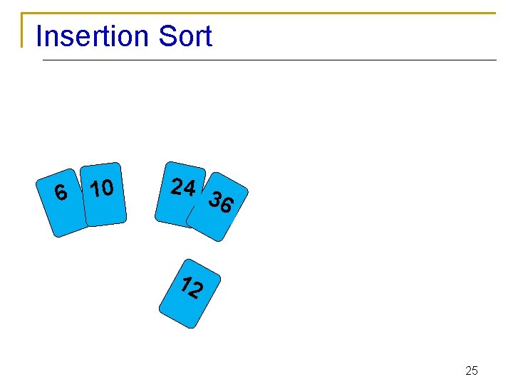
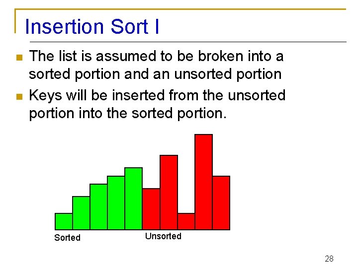
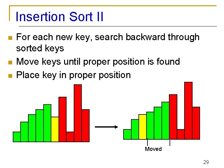
Insertion Sort n Idea: like sorting a hand of playing cards q q Start with an empty left hand the cards facing down on the table. Remove one card at a time from the table, and insert it into the correct position in the left hand n q compare it with each of the cards already in the hand, from right to left The cards held in the left hand are sorted n these cards were originally the top cards of the pile on the table 22

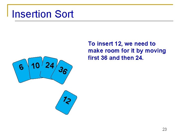
Insertion Sort 2 4 3 0 1 6 6 To insert 12, we need to make room for it by moving first 36 and then 24. 12 23

Insertion Sort 2 4 0 1 6 36 12 24

Insertion Sort 6 10 24 3 6 12 25

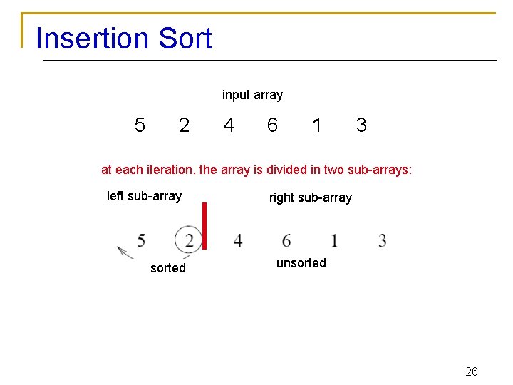
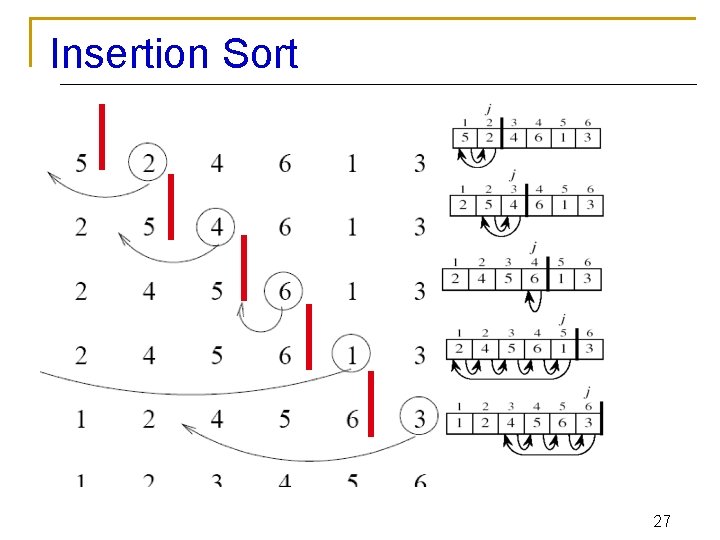
Insertion Sort input array 5 2 4 6 1 3 at each iteration, the array is divided in two sub-arrays: left sub-array sorted right sub-array unsorted 26

Insertion Sort 27

Insertion Sort I n n The list is assumed to be broken into a sorted portion and an unsorted portion Keys will be inserted from the unsorted portion into the sorted portion. Sorted Unsorted 28

Insertion Sort II n n n For each new key, search backward through sorted keys Move keys until proper position is found Place key in proper position Moved 29

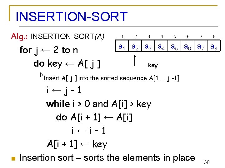
INSERTION-SORT Alg. : INSERTION-SORT(A) for j ← 2 to n do key ← A[ j ] 1 2 3 4 5 6 7 8 a 1 a 2 a 3 a 4 a 5 a 6 a 7 a 8 key Insert A[ j ] into the sorted sequence A[1. . j -1] n i←j-1 while i > 0 and A[i] > key do A[i + 1] ← A[i] i←i– 1 A[i + 1] ← key Insertion sort – sorts the elements in place 30

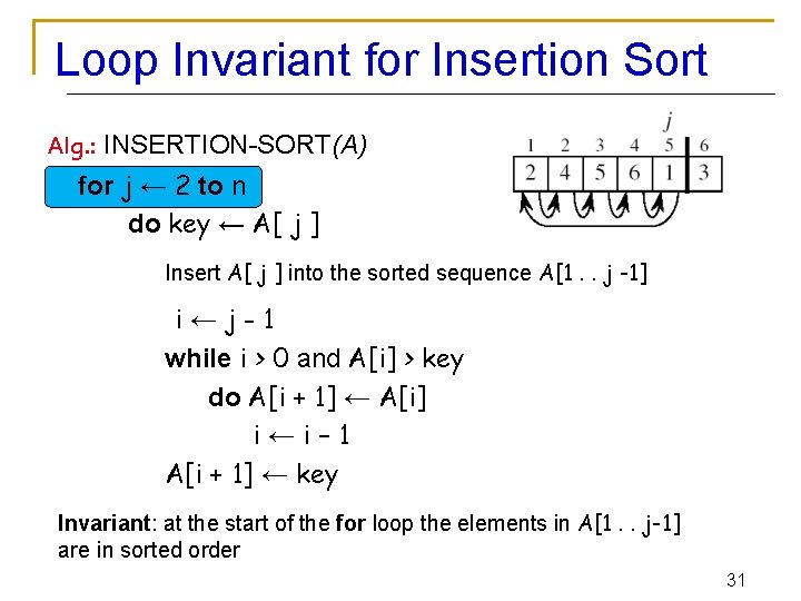
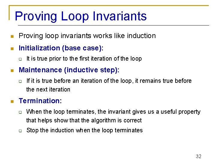
Loop Invariant for Insertion Sort Alg. : INSERTION-SORT(A) for j ← 2 to n do key ← A[ j ] Insert A[ j ] into the sorted sequence A[1. . j -1] i←j-1 while i > 0 and A[i] > key do A[i + 1] ← A[i] i←i– 1 A[i + 1] ← key Invariant: at the start of the for loop the elements in A[1. . j-1] are in sorted order 31

Proving Loop Invariants n Proving loop invariants works like induction n Initialization (base case): q n Maintenance (inductive step): q n It is true prior to the first iteration of the loop If it is true before an iteration of the loop, it remains true before the next iteration Termination: q q When the loop terminates, the invariant gives us a useful property that helps show that the algorithm is correct Stop the induction when the loop terminates 32

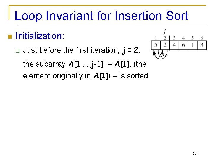
Loop Invariant for Insertion Sort n Initialization: q Just before the first iteration, j = 2: the subarray A[1. . j-1] = A[1], (the element originally in A[1]) – is sorted 33

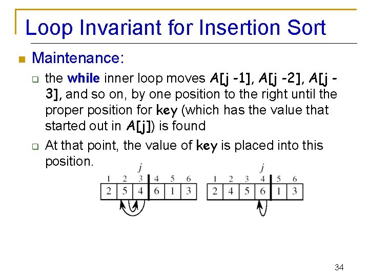
Loop Invariant for Insertion Sort n Maintenance: q q the while inner loop moves A[j -1], A[j -2], A[j 3], and so on, by one position to the right until the proper position for key (which has the value that started out in A[j]) is found At that point, the value of key is placed into this position. 34

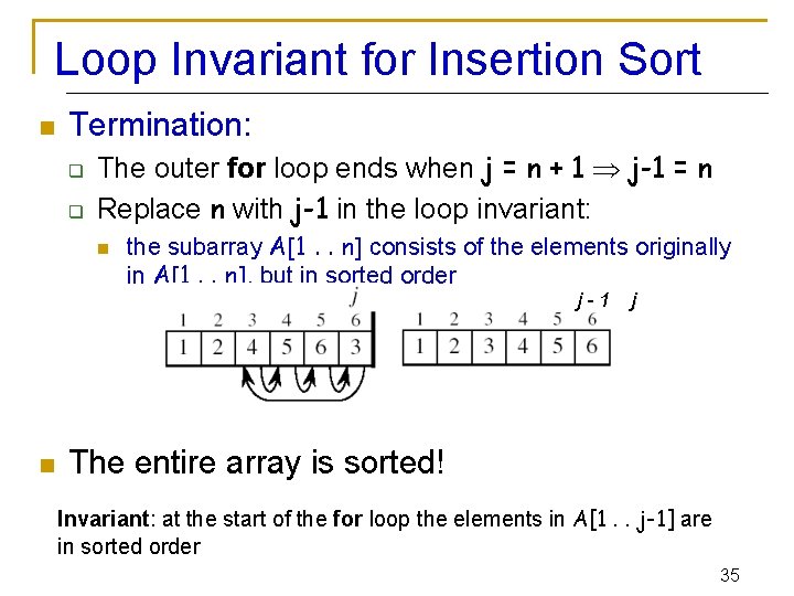
Loop Invariant for Insertion Sort n Termination: q q The outer for loop ends when j = n + 1 j-1 = n Replace n with j-1 in the loop invariant: n the subarray A[1. . n] consists of the elements originally in A[1. . n], but in sorted order j-1 n j The entire array is sorted! Invariant: at the start of the for loop the elements in A[1. . j-1] are in sorted order 35

Analysis of Insertion Sort INSERTION-SORT(A) cost c 1 c 2 Insert A[ j ] into the sorted sequence A[1. . j -1] 0 i ← j - 1 Worst case i-1 comparisons c 4 c 5 while i > 0 and A[i] > key c 6 do A[i + 1] ← A[i] c 7 i←i– 1 c 8 A[i + 1] ← key for j ← 2 to n do key ← A[ j ] Fixed n-1 iterations times n n-1 n-1 tj: # of times the while statement is executed at iteration j 36

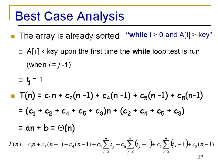
Best Case Analysis n The array is already sorted “while i > 0 and A[i] > key” q A[i] ≤ key upon the first time the while loop test is run (when i = j -1) q n tj = 1 T(n) = c 1 n + c 2(n -1) + c 4(n -1) + c 5(n -1) + c 8(n-1) = (c 1 + c 2 + c 4 + c 5 + c 8)n + (c 2 + c 4 + c 5 + c 8) = an + b = (n) 37

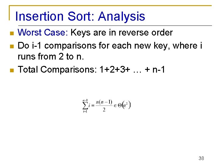
Insertion Sort: Analysis n n n Worst Case: Keys are in reverse order Do i-1 comparisons for each new key, where i runs from 2 to n. Total Comparisons: 1+2+3+ … + n-1 38

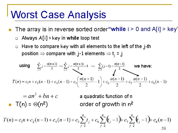
Worst Case Analysis n The array is in reverse sorted order “while i > 0 and A[i] > key” q q Always A[i] > key in while loop test Have to compare key with all elements to the left of the j-th position compare with j-1 elements tj = j using we have: a quadratic function of n n T(n) = (n 2) order of growth in n 2 39

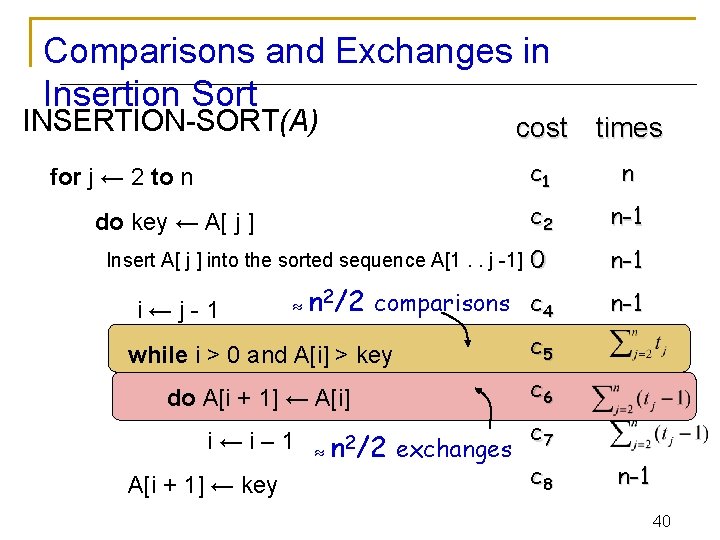
Comparisons and Exchanges in Insertion Sort INSERTION-SORT(A) cost times c 1 n c 2 n-1 0 n-1 comparisons c 4 n-1 for j ← 2 to n do key ← A[ j ] Insert A[ j ] into the sorted sequence A[1. . j -1] i←j-1 n 2/2 while i > 0 and A[i] > key c 5 do A[i + 1] ← A[i] c 6 i←i– 1 A[i + 1] ← key n 2/2 exchanges c 7 c 8 n-1 40

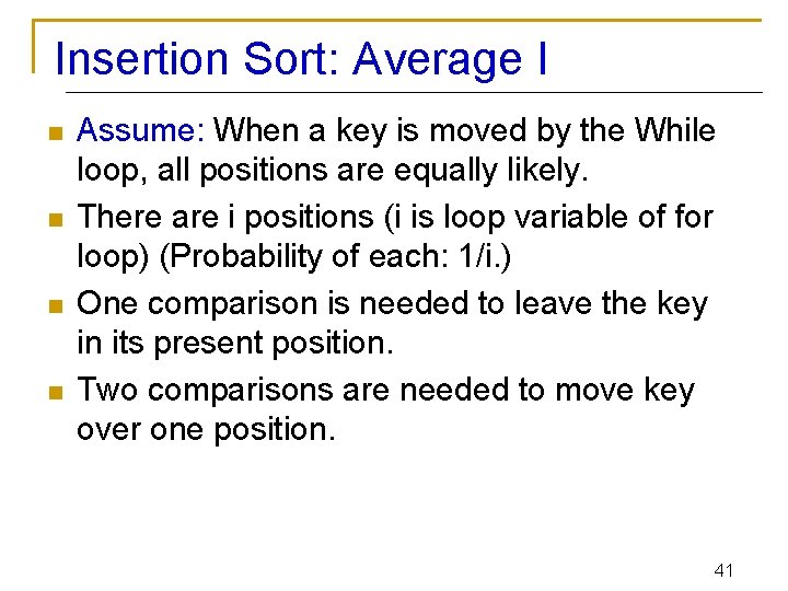
Insertion Sort: Average I n n Assume: When a key is moved by the While loop, all positions are equally likely. There are i positions (i is loop variable of for loop) (Probability of each: 1/i. ) One comparison is needed to leave the key in its present position. Two comparisons are needed to move key over one position. 41

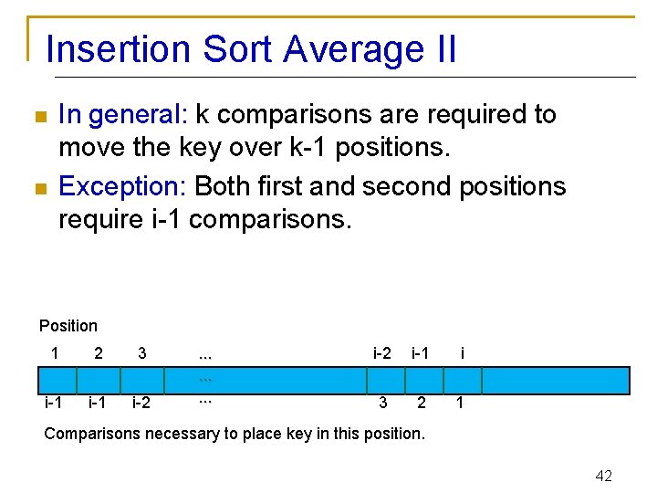
Insertion Sort Average II n n In general: k comparisons are required to move the key over k-1 positions. Exception: Both first and second positions require i-1 comparisons. Position 1 2 3 i-1 i-2 . . i-2 i-1 i 3 2 1 Comparisons necessary to place key in this position. 42

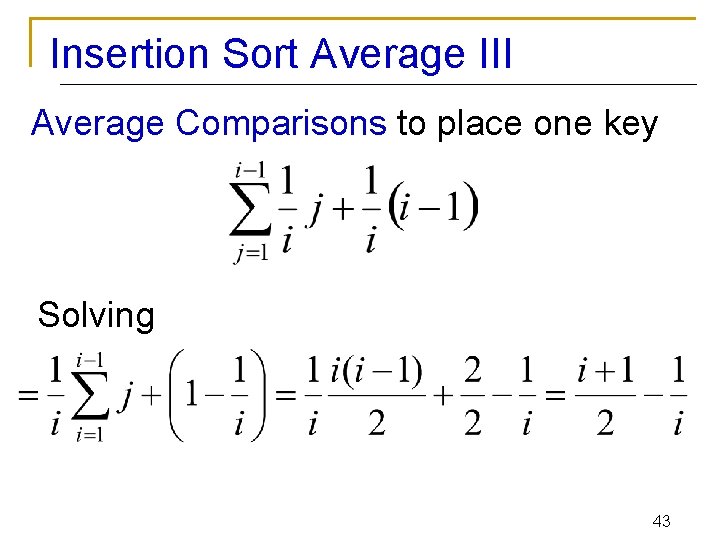
Insertion Sort Average III Average Comparisons to place one key Solving 43

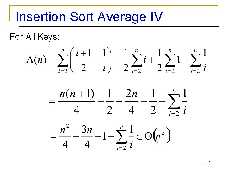
Insertion Sort Average IV For All Keys: 44

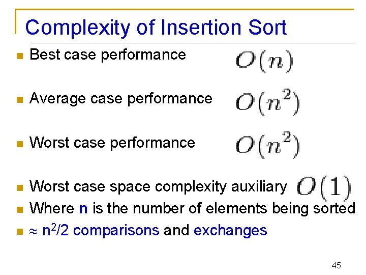
Complexity of Insertion Sort n Best case performance n Average case performance n Worst case space complexity auxiliary Where n is the number of elements being sorted n 2/2 comparisons and exchanges n n 45

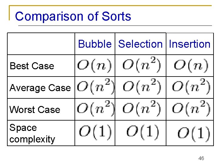
Comparison of Sorts Bubble Selection Insertion Best Case Average Case Worst Case Space complexity 46

Comparison Bubble and Insertion n Sort Bubble sort is asymptotically equivalent in n running time O(n 2) to insertion sort in the worst case But the two algorithms differ greatly in the number of swaps necessary Experimental results have also shown that insertion sort performs considerably better even on random lists. For these reasons many modern algorithm textbooks avoid using the bubble sort algorithm in favor of insertion sort. 47

Comparison Bubble and Insertion n Sort Bubble sort also interacts poorly with modern CPU hardware. It requires q q q n at least twice as many writes as insertion sort, twice as many cache misses, and asymptotically more branch miss predictions. Experiments of sorting strings in Java show bubble sort to be q q roughly 5 times slower than insertion sort and 40% slower than selection sort 48

Comparison of Selection Sort n n n Among simple average-case Θ(n 2) algorithms, selection sort almost always outperforms bubble sort Simple calculation shows that insertion sort will therefore usually perform about half as many comparisons as selection sort, although it can perform just as many or far fewer depending on the order the array was in prior to sorting selection sort is preferable to insertion sort in terms of number of writes (Θ(n) swaps versus Ο(n 2) swaps) 49

Optimality Analysis I n n n To discover an optimal algorithm we need to find an upper and lower asymptotic bound for a problem. An algorithm gives us an upper bound. The worst case for sorting cannot exceed (n 2) because we have Insertion Sort that runs that fast. Lower bounds require mathematical arguments 50

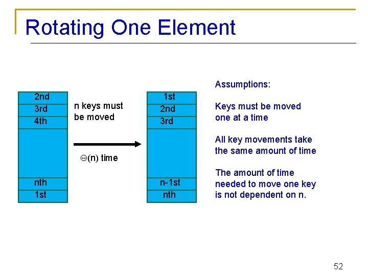
Optimality Analysis II n n n Making mathematical arguments usually involves assumptions about how the problem will be solved. Invalidating the assumptions invalidates the lower bound. Sorting an array of numbers requires at least (n) time, because it would take that much time to rearrange a list that was rotated one element out of position. 51

Rotating One Element Assumptions: 2 nd 3 rd 4 th n keys must be moved 1 st 2 nd 3 rd All key movements take the same amount of time (n) time nth 1 st Keys must be moved one at a time n-1 st nth The amount of time needed to move one key is not dependent on n. 52

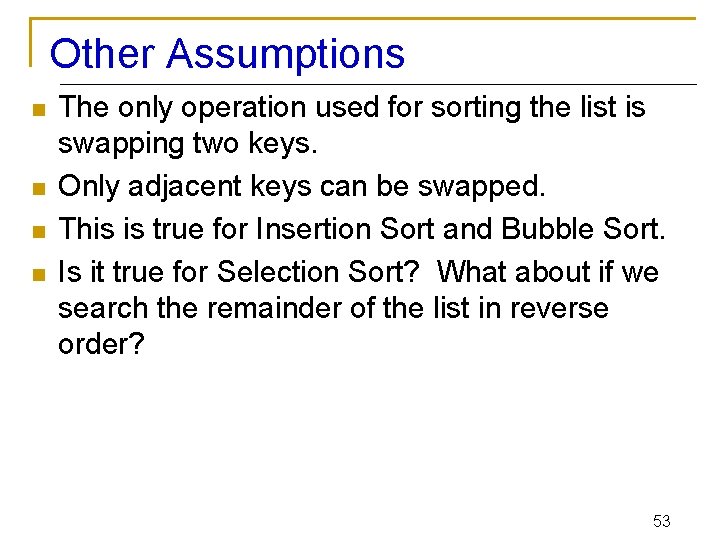
Other Assumptions n n The only operation used for sorting the list is swapping two keys. Only adjacent keys can be swapped. This is true for Insertion Sort and Bubble Sort. Is it true for Selection Sort? What about if we search the remainder of the list in reverse order? 53

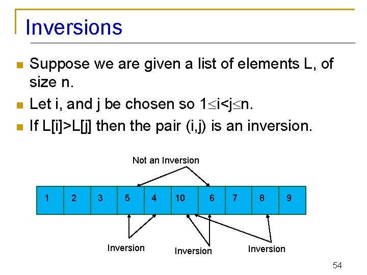
Inversions n n n Suppose we are given a list of elements L, of size n. Let i, and j be chosen so 1 i<j n. If L[i]>L[j] then the pair (i, j) is an inversion. Not an Inversion 1 2 3 5 Inversion 4 10 6 Inversion 7 8 9 Inversion 54

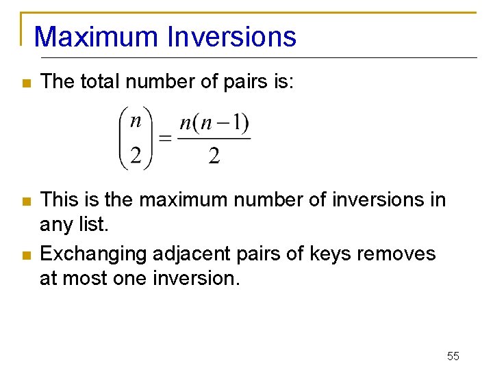
Maximum Inversions n The total number of pairs is: n This is the maximum number of inversions in any list. Exchanging adjacent pairs of keys removes at most one inversion. n 55

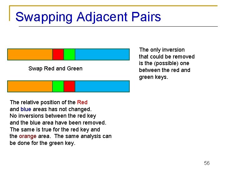
Swapping Adjacent Pairs Swap Red and Green The only inversion that could be removed is the (possible) one between the red and green keys. The relative position of the Red and blue areas has not changed. No inversions between the red key and the blue area have been removed. The same is true for the red key and the orange area. The same analysis can be done for the green key. 56

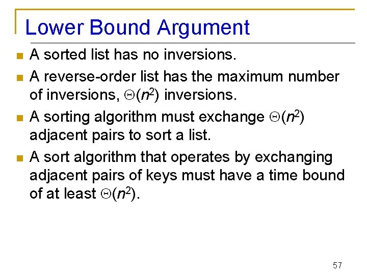
Lower Bound Argument n n A sorted list has no inversions. A reverse-order list has the maximum number of inversions, (n 2) inversions. A sorting algorithm must exchange (n 2) adjacent pairs to sort a list. A sort algorithm that operates by exchanging adjacent pairs of keys must have a time bound of at least (n 2). 57

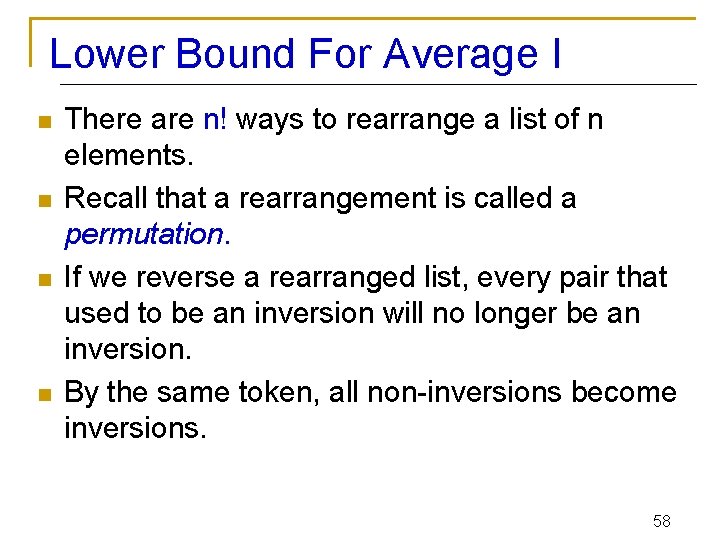
Lower Bound For Average I n n There are n! ways to rearrange a list of n elements. Recall that a rearrangement is called a permutation. If we reverse a rearranged list, every pair that used to be an inversion will no longer be an inversion. By the same token, all non-inversions become inversions. 58

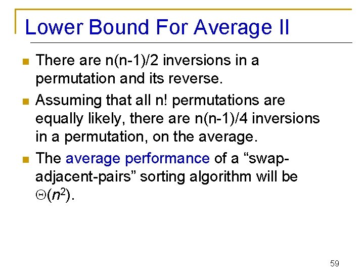
Lower Bound For Average II n n n There are n(n-1)/2 inversions in a permutation and its reverse. Assuming that all n! permutations are equally likely, there are n(n-1)/4 inversions in a permutation, on the average. The average performance of a “swapadjacent-pairs” sorting algorithm will be (n 2). 59

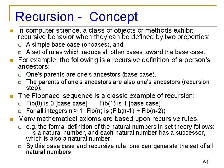
Recursion n is the process of repeating items in a selfsimilar way. For instance, when the surfaces of two mirrors are exactly parallel with each other the nested images that occur are a form of infinite recursion. The term recursion has a variety of meanings specific to a variety of disciplines ranging from linguistics to logic. 60

Recursion - Concept n In computer science, a class of objects or methods exhibit recursive behavior when they can be defined by two properties: q q n For example, the following is a recursive definition of a person's ancestors: q q n One's parents are one's ancestors (base case). The parents of one's ancestors are also one's ancestors (recursion step). The Fibonacci sequence is a classic example of recursion: q q n A simple base case (or cases), and A set of rules which reduce all other cases toward the base case. Fib(0) is 0 [base case] Fib(1) is 1 [base case] For all integers n > 1: Fib(n) is (Fib(n-1) + Fib(n-2)) Many mathematical axioms are based upon recursive rules. q q e. g. the formal definition of the natural numbers in set theory follows: 1 is a natural number, and each natural number has a successor, which is also a natural number. By this base case and recursive rule, one can generate the set of all natural numbers 61

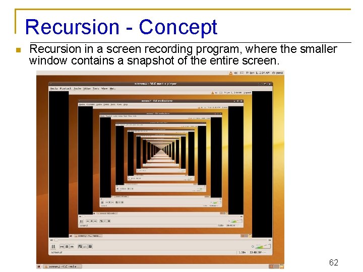
Recursion - Concept n Recursion in a screen recording program, where the smaller window contains a snapshot of the entire screen. 62

Recursion n n It is a method where the solution to a problem depends on solutions to smaller instances of the same problem The approach can be applied to many types of problems, and is one of the central ideas of computer science The power of recursion evidently lies in the possibility of defining an infinite set of objects by a finite statement. In the same manner, an infinite number of computations can be described by a finite recursive program, even if this program contains no explicit repetitions 63

Recursion n Most computer programming languages support recursion by allowing a function to call itself within the program text Some functional programming languages do not define any looping constructs but rely solely on recursion to repeatedly call code Computability theory has proven that these recursive-only languages are mathematically equivalent to the imperative languages q meaning they can solve the same kinds of problems even without the typical control structures like “while” and “for” 64 64

Recursive Algorithms n A common computer programming tactic is q q q n When combined with a lookup table that stores the results of solving sub-problems q n to divide a problem into sub-problems of the same type as the original, solve those problems, and combine the results This is often referred to as the divide-and-conquer method (to avoid solving them repeatedly and incurring extra computation time) It can be referred to as dynamic programming 65

Recursive Function n A recursive function definition has one or more base cases q q n meaning input(s) for which the function produces a result trivially (without recurring), and one or more recursive cases, meaning input(s) for which the program recurs (calls itself). For example, the factorial function can be defined recursively by the equations 0! = 1 and, for all n >0; n! = n(n-1)! Neither equation by itself constitutes a complete definition; q q First is the base case, and Second is the recursive case. 66

Recursive Function n The job of the recursive cases can be seen as breaking down complex inputs into simpler ones In a properly designed recursive function, with each recursive call, the input problem must be simplified in such a way that eventually the base case must be reached. Neglecting to write a base case, or testing for it incorrectly, can cause an infinite loop 67

Recursion n Recursive functions q q q Function that calls itself Can only solve a base case Divides up problem into n n n What it can do What it cannot do - resembles original problem q Launches a new copy of itself (recursion step) Eventually base case gets solved q Gets plugged in, works its way up and solves whole problem 68

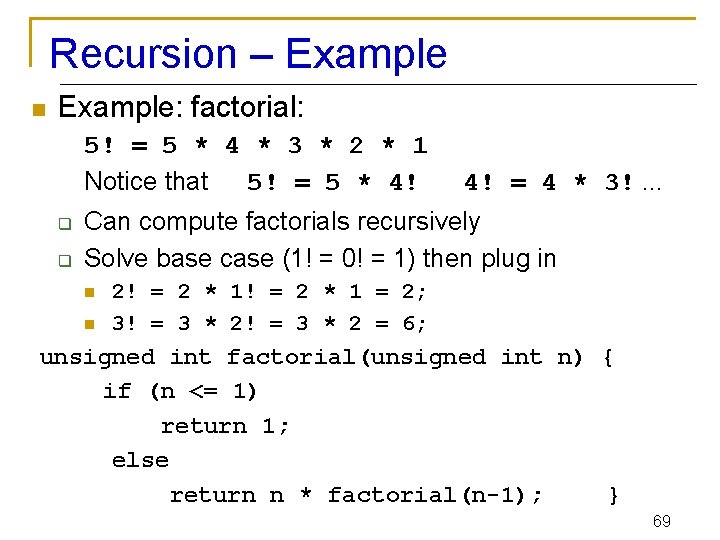
Recursion – Example n Example: factorial: 5! = 5 * 4 * 3 * 2 * 1 Notice that 5! = 5 * 4! q q 4! = 4 * 3!. . . Can compute factorials recursively Solve base case (1! = 0! = 1) then plug in n n 2! = 2 * 1 = 2; 3! = 3 * 2 = 6; unsigned int factorial(unsigned int n) { if (n <= 1) return 1; else return n * factorial(n-1); } 69

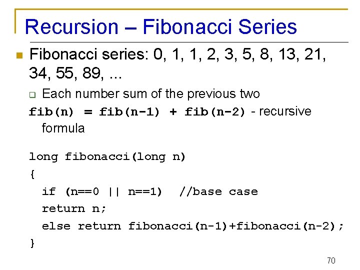
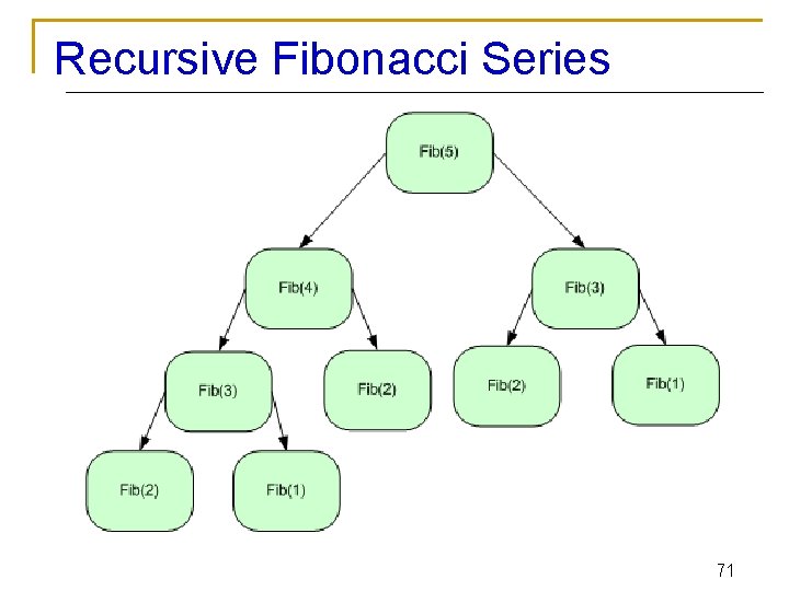
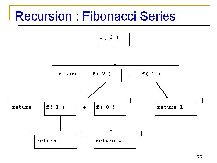
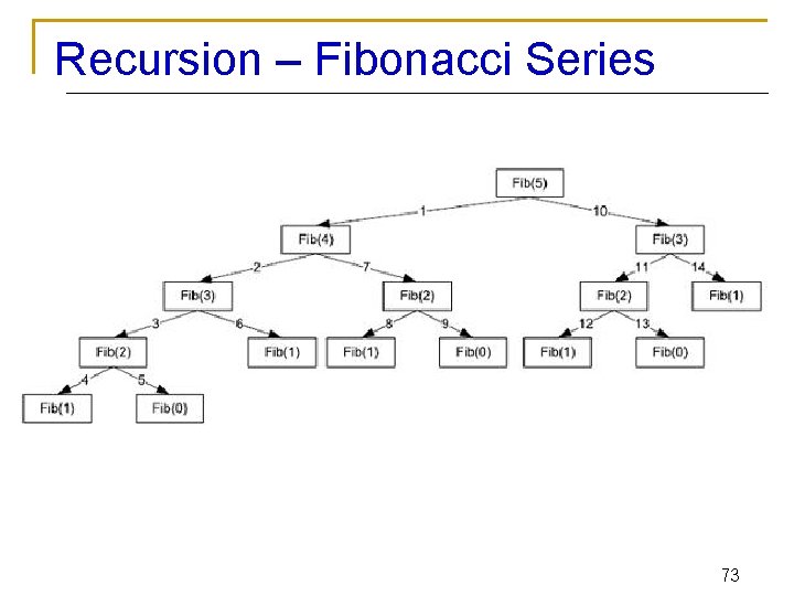
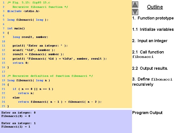
Recursion – Fibonacci Series n Fibonacci series: 0, 1, 1, 2, 3, 5, 8, 13, 21, 34, 55, 89, . . . Each number sum of the previous two fib(n) = fib(n-1) + fib(n-2) - recursive formula q long fibonacci(long n) { if (n==0 || n==1) //base case return n; else return fibonacci(n-1)+fibonacci(n-2); } 70

Recursive Fibonacci Series 71

Recursion : Fibonacci Series f( 3 ) return f( 1 ) return 1 f( 2 ) + f( 0 ) + f( 1 ) return 1 return 0 72

Recursion – Fibonacci Series 73

1 2 3 4 5 6 7 8 9 10 11 12 13 14 15 16 17 18 19 20 21 22 23 24 25 /* Fig. 5. 15: fig 05_15. c Recursive fibonacci function */ #include <stdio. h> long fibonacci( long ); int main() { long result, number; printf( "Enter an integer: " ); scanf( "%ld", &number ); result = fibonacci( number ); printf( "Fibonacci( %ld ) = %ldn", number, result ); return 0; } /* Recursive definition of function fibonacci */ long fibonacci( long n ) { if ( n == 0 || n == 1 ) return n; else return fibonacci( n - 1 ) + fibonacci( n - 2 ); } Enter an integer: 0 Fibonacci(0) = 0 Enter an integer: 1 Fibonacci(1) = 1 2000 Prentice Hall, Inc. All rights reserved. Outline 1. Function prototype 1. 1 Initialize variables 2. Input an integer 2. 1 Call function fibonacci 2. 2 Output results. 3. Define fibonacci recursively Program Output

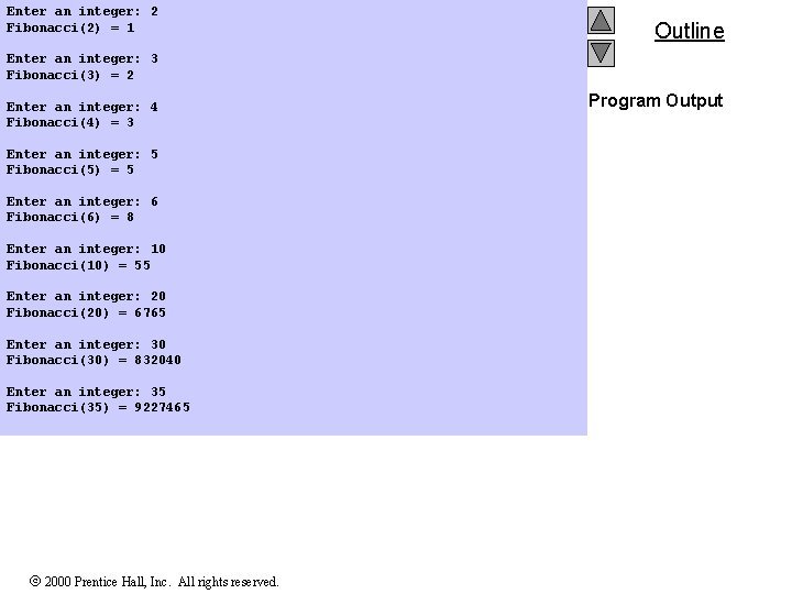
Enter an integer: 2 Fibonacci(2) = 1 Outline Enter an integer: 3 Fibonacci(3) = 2 Enter an integer: 4 Fibonacci(4) = 3 Enter an integer: 5 Fibonacci(5) = 5 Enter an integer: 6 Fibonacci(6) = 8 Enter an integer: 10 Fibonacci(10) = 55 Enter an integer: 20 Fibonacci(20) = 6765 Enter an integer: 30 Fibonacci(30) = 832040 Enter an integer: 35 Fibonacci(35) = 9227465 2000 Prentice Hall, Inc. All rights reserved. Program Output

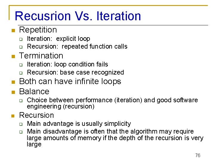
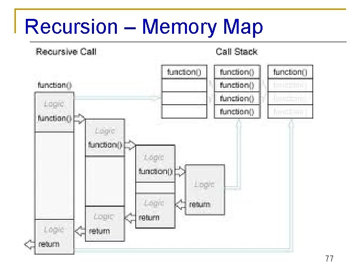
Recusrion Vs. Iteration n Repetition q q n Termination q q n n Iteration: loop condition fails Recursion: base case recognized Both can have infinite loops Balance q n Iteration: explicit loop Recursion: repeated function calls Choice between performance (iteration) and good software engineering (recursion) Recursion q q Main advantage is usually simplicity Main disadvantage is often that the algorithm may require large amounts of memory if the depth of the recursion is very large 76

Recursion – Memory Map 77

Summary n Comparison of Sorting methods Bubble, q Selection and q Insertion q n Recursion Concept q Example q Implementation Code q 78