CS 685 G Special Topics in Data Mining

CS 685 G: Special Topics in Data Mining Hierarchical Clustering Analysis Jinze Liu

Clustering Presentation Topics • Topic 1 – X-means – Learning the k in k-means – https: //papers. nips. cc/paper/2526 -learning-the-k-in-k-means. pdf • Topic 2 – Co-clustering – https: //pdfs. semanticscholar. org/4 a 3 e/b 95 f 17 a 88 e 14227 b 05 a 590639 e 8 c d 3346 a 99. pdf • Topic 3 – https: //web. cse. ohio-state. edu/~jwdavis/Publications/cvpr 11 a. pdf

Outline • • What is clustering Partitioning methods Hierarchical methods Density-based methods Grid-based methods Model-based clustering methods Outlier analysis

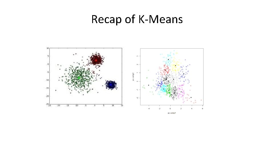
Recap of K-Means

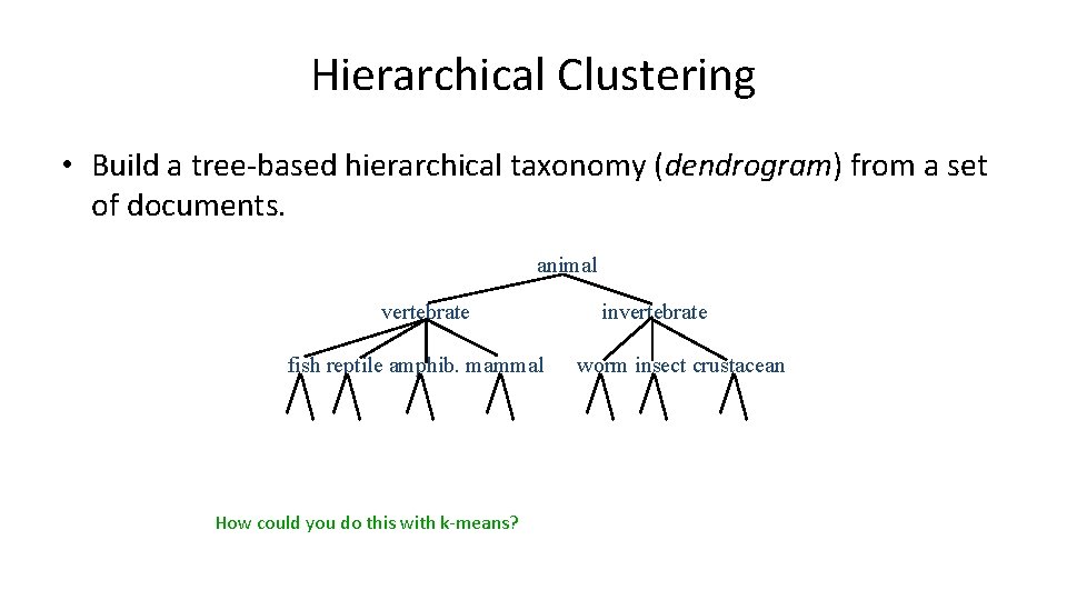
Hierarchical Clustering • Build a tree-based hierarchical taxonomy (dendrogram) from a set of documents. animal vertebrate fish reptile amphib. mammal How could you do this with k-means? invertebrate worm insect crustacean

Hierarchical Clustering algorithms • Agglomerative (bottom-up): – Start with each document being a single cluster. – Eventually all documents belong to the same cluster. • Divisive (top-down): – Start with all documents belong to the same cluster. – Eventually each node forms a cluster on its own. – Could be a recursive application of k-means like algorithms • Does not require the number of clusters k in advance • Needs a termination/readout condition

Hierarchical Agglomerative Clustering (HAC) • Assumes a similarity function for determining the similarity of two instances. • Starts with all instances in a separate cluster and then repeatedly joins the two clusters that are most similar until there is only one cluster. • The history of merging forms a binary tree or hierarchy.

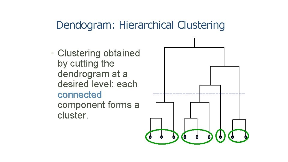
Dendogram: Hierarchical Clustering • Clustering obtained by cutting the dendrogram at a desired level: each connected component forms a cluster.

Hierarchical Agglomerative Clustering (HAC) • Starts with each doc in a separate cluster – then repeatedly joins the closest pair of clusters, until there is only one cluster. • The history of merging forms a binary tree or hierarchy. How to measure distance of clusters? ?

Closest pair of clusters Many variants to defining closest pair of clusters • Single-link – Distance of the “closest” points (single-link) • Complete-link – Distance of the “furthest” points • Centroid – Distance of the centroids (centers of gravity) • (Average-link) – Average distance between pairs of elements

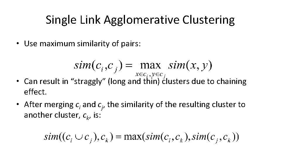
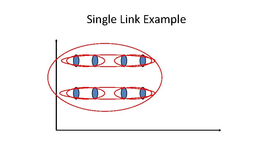
Single Link Agglomerative Clustering • Use maximum similarity of pairs: • Can result in “straggly” (long and thin) clusters due to chaining effect. • After merging ci and cj, the similarity of the resulting cluster to another cluster, ck, is:

Single Link Example

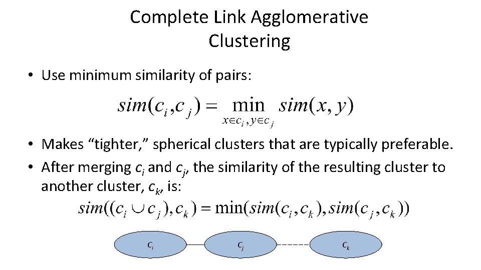
Complete Link Agglomerative Clustering • Use minimum similarity of pairs: • Makes “tighter, ” spherical clusters that are typically preferable. • After merging ci and cj, the similarity of the resulting cluster to another cluster, ck, is: Ci Cj Ck

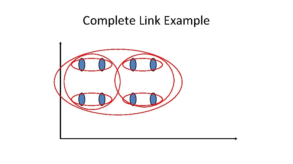
Complete Link Example

Key notion: cluster representative • We want a notion of a representative point in a cluster • Representative should be some sort of “typical” or central point in the cluster, e. g. , – point inducing smallest radii to docs in cluster – smallest squared distances, etc. – point that is the “average” of all docs in the cluster • Centroid or center of gravity

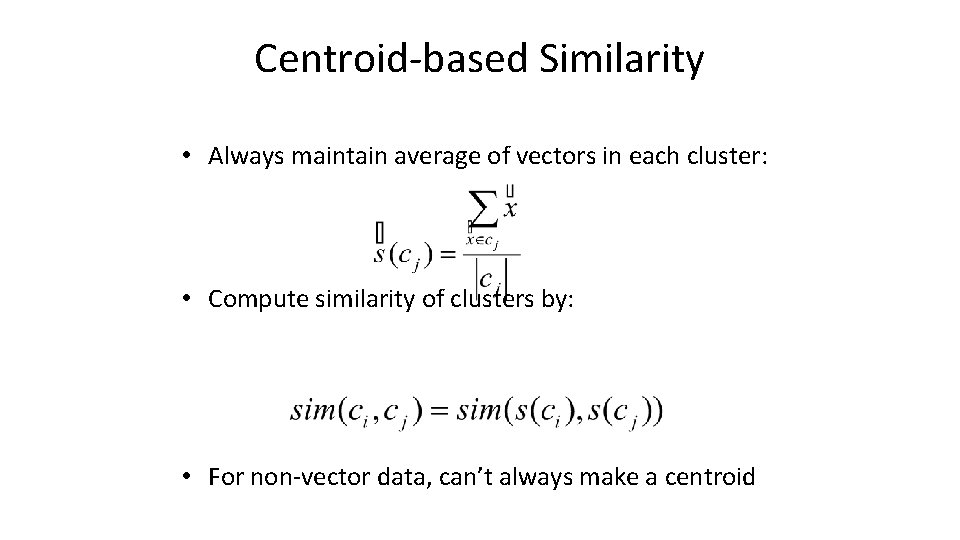
Centroid-based Similarity • Always maintain average of vectors in each cluster: • Compute similarity of clusters by: • For non-vector data, can’t always make a centroid

Computational Complexity • In the first iteration, all HAC methods need to compute similarity of all pairs of n individual instances which is O(mn 2). • In each of the subsequent n 2 merging iterations, compute the distance between the most recently created cluster and all other existing clusters. • Maintaining of heap of distances allows this to be O(mn 2 logn)

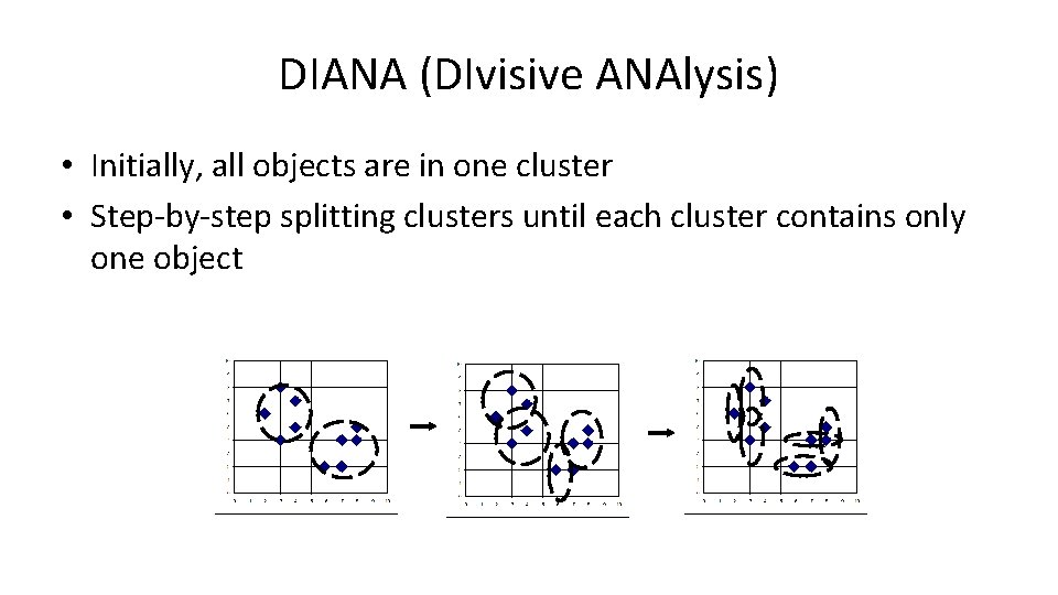
DIANA (DIvisive ANAlysis) • Initially, all objects are in one cluster • Step-by-step splitting clusters until each cluster contains only one object

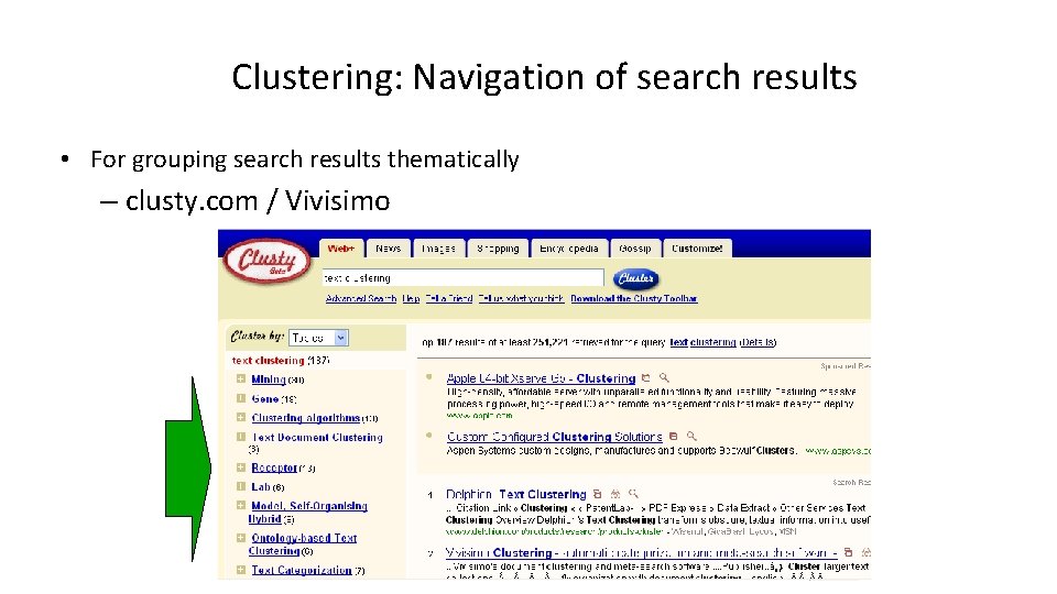
Clustering: Navigation of search results • For grouping search results thematically – clusty. com / Vivisimo

Major issue - labeling • After clustering algorithm finds clusters - how can they be useful to the end user? • Need pithy label for each cluster – In search results, say “Animal” or “Car” in the jaguar example. – In topic trees, need navigational cues. • Often done by hand, a posteriori. How would you do this?

How to Label Clusters • Show titles of typical documents – Titles are easy to scan – Authors create them for quick scanning! – But you can only show a few titles which may not fully represent cluster • Show words/phrases prominent in cluster – More likely to fully represent cluster – Use distinguishing words/phrases • Differential labeling – But harder to scan

Labeling • Common heuristics - list 5 -10 most frequent terms in the centroid vector. – Drop stop-words; stem. • Differential labeling by frequent terms – Within a collection “Computers”, clusters all have the word computer as frequent term. – Discriminant analysis of centroids. • Perhaps better: distinctive noun phrase

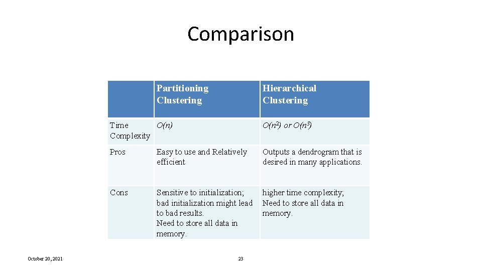
Comparison Partitioning Clustering October 20, 2021 Hierarchical Clustering Time O(n) Complexity O(n 2) or O(n 3) Pros Easy to use and Relatively efficient Outputs a dendrogram that is desired in many applications. Cons Sensitive to initialization; bad initialization might lead to bad results. Need to store all data in memory. higher time complexity; Need to store all data in memory. 23

Other Alternatives • Integrating hierarchical clustering with other techniques – BIRCH, CURE, CHAMELEON, ROCK

BIRCH Balanced Iterative Reducing and Clustering using Hierarchies

Introduction to BIRCH • Designed for very large data sets – – Time and memory are limited Incremental and dynamic clustering of incoming objects Only one scan of data is necessary Does not need the whole data set in advance • Two key phases: – Scans the database to build an in-memory tree – Applies clustering algorithm to cluster the leaf nodes October 20, 2021 26

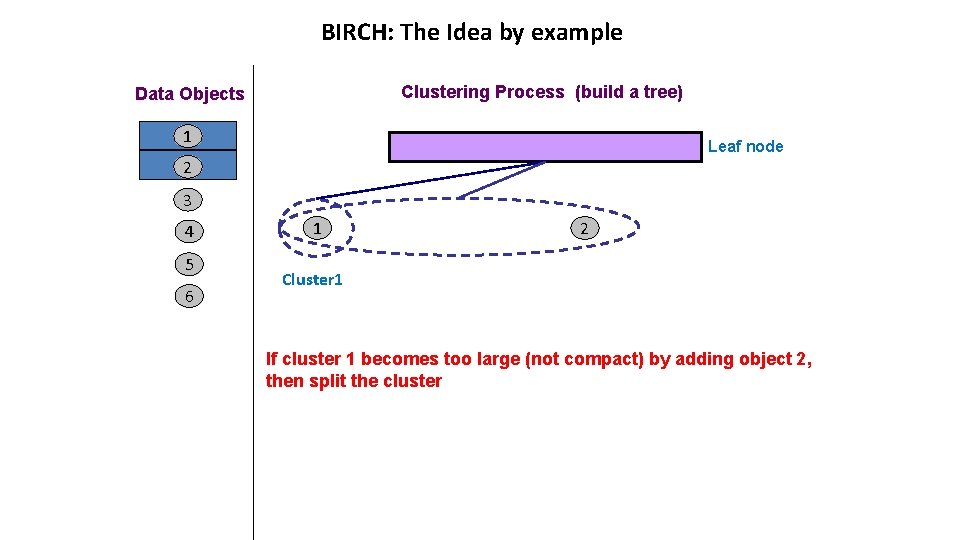
BIRCH: The Idea by example Clustering Process (build a tree) Data Objects 1 Leaf node 2 3 4 5 6 1 2 Cluster 1 If cluster 1 becomes too large (not compact) by adding object 2, then split the cluster

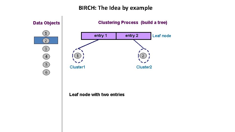
BIRCH: The Idea by example Clustering Process (build a tree) Data Objects 1 entry 2 Leaf node 2 3 4 5 1 2 Cluster 1 Cluster 2 6 Leaf node with two entries

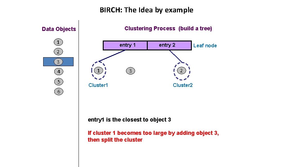
BIRCH: The Idea by example Clustering Process (build a tree) Data Objects 1 entry 2 Leaf node 2 3 4 5 1 3 Cluster 1 2 Cluster 2 6 entry 1 is the closest to object 3 If cluster 1 becomes too large by adding object 3, then split the cluster

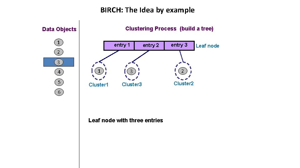
BIRCH: The Idea by example Clustering Process (build a tree) Data Objects 1 entry 2 entry 3 2 3 4 1 3 2 5 Cluster 1 Cluster 3 Cluster 2 6 Leaf node with three entries Leaf node

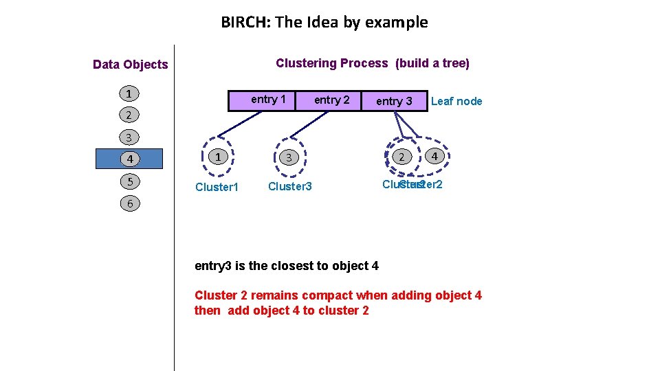
BIRCH: The Idea by example Clustering Process (build a tree) Data Objects 1 entry 1 2 entry 3 Leaf node 3 4 1 3 5 Cluster 1 Cluster 3 2 4 Cluster 2 6 entry 3 is the closest to object 4 Cluster 2 remains compact when adding object 4 then add object 4 to cluster 2

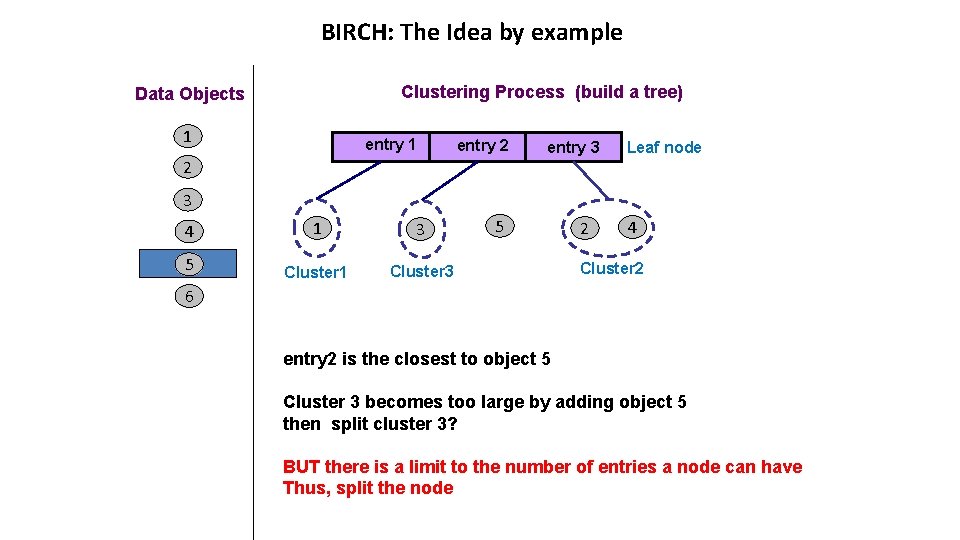
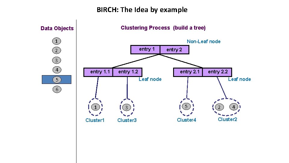
BIRCH: The Idea by example Clustering Process (build a tree) Data Objects 1 entry 2 2 entry 3 Leaf node 3 4 1 3 5 Cluster 1 Cluster 3 5 2 4 Cluster 2 6 entry 2 is the closest to object 5 Cluster 3 becomes too large by adding object 5 then split cluster 3? BUT there is a limit to the number of entries a node can have Thus, split the node

BIRCH: The Idea by example Clustering Process (build a tree) Data Objects 1 Non-Leaf node entry 1 2 entry 2 3 4 entry 1. 1 entry 2. 1 entry 1. 2 5 entry 2. 2 Leaf node 6 1 3 5 Cluster 1 Cluster 3 Cluster 4 2 4 Cluster 2

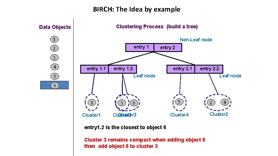
BIRCH: The Idea by example Clustering Process (build a tree) Data Objects 1 Non-Leaf node entry 1 2 entry 2 3 4 entry 1. 1 entry 2. 1 entry 1. 2 5 entry 2. 2 Leaf node 6 1 Cluster 1 3 6 Cluster 3 5 Cluster 4 entry 1. 2 is the closest to object 6 Cluster 3 remains compact when adding object 6 then add object 6 to cluster 3 2 4 Cluster 2

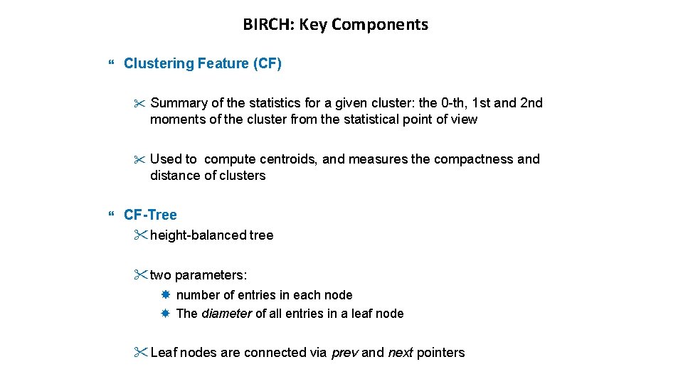
BIRCH: Key Components Clustering Feature (CF) " Summary of the statistics for a given cluster: the 0 -th, 1 st and 2 nd moments of the cluster from the statistical point of view " Used to compute centroids, and measures the compactness and distance of clusters CF-Tree "height-balanced tree "two parameters: number of entries in each node The diameter of all entries in a leaf node "Leaf nodes are connected via prev and next pointers

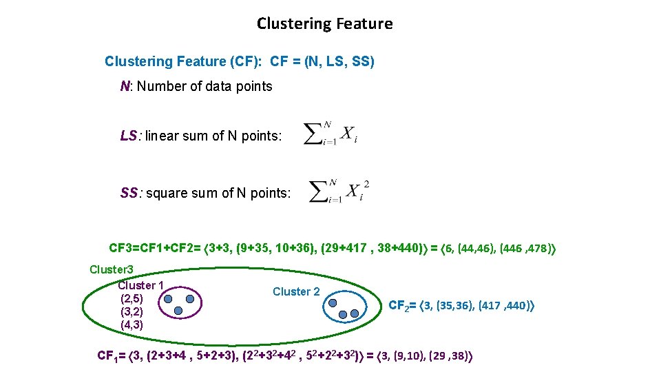
Clustering Feature (CF): CF = (N, LS, SS) N: Number of data points LS: linear sum of N points: SS: square sum of N points: CF 3=CF 1+CF 2= 3+3, (9+35, 10+36), (29+417 , 38+440) = 6, (44, 46), (446 , 478) Cluster 3 Cluster 1 (2, 5) (3, 2) (4, 3) Cluster 2 CF 2= 3, (35, 36), (417 , 440) CF 1= 3, (2+3+4 , 5+2+3), (22+32+42 , 52+22+32) = 3, (9, 10), (29 , 38)

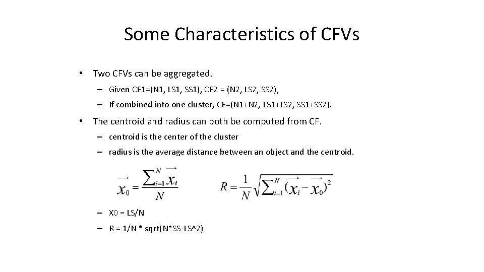
Some Characteristics of CFVs • Two CFVs can be aggregated. – Given CF 1=(N 1, LS 1, SS 1), CF 2 = (N 2, LS 2, SS 2), – If combined into one cluster, CF=(N 1+N 2, LS 1+LS 2, SS 1+SS 2). • The centroid and radius can both be computed from CF. – centroid is the center of the cluster – radius is the average distance between an object and the centroid. – X 0 = LS/N – R = 1/N * sqrt(N*SS-LS^2)

Clustering Feature • Clustering feature: – Summarize the statistics for a subcluster • the 0 th, 1 st and 2 nd moments of the subcluster – Register crucial measurements for computing cluster and utilize storage efficiently

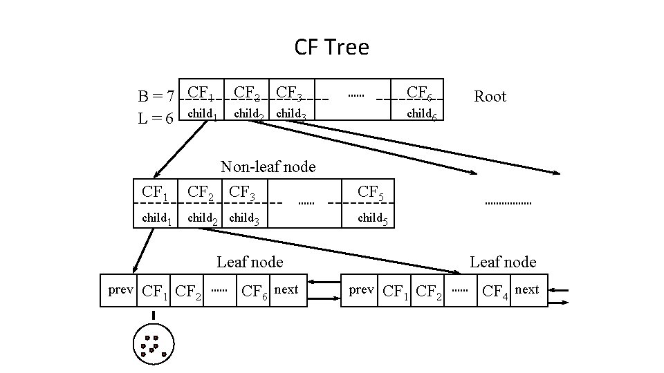
CF-tree in BIRCH • A CF tree: a height-balanced tree storing the clustering features for a hierarchical clustering – A nonleaf node in a tree has descendants or “children” – The nonleaf nodes store sums of the CFs of children

CF Tree B = 7 CF 1 CF 2 CF 3 L = 6 child 1 child 2 child 3 CF 6 child 6 CF 1 Non-leaf node CF 2 CF 3 CF 5 child 1 child 2 child 3 child 5 Leaf node prev CF 1 CF 2 CF 6 next Root Leaf node prev CF 1 CF 2 CF 4 next

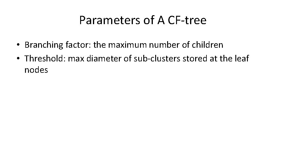
Parameters of A CF-tree • Branching factor: the maximum number of children • Threshold: max diameter of sub-clusters stored at the leaf nodes

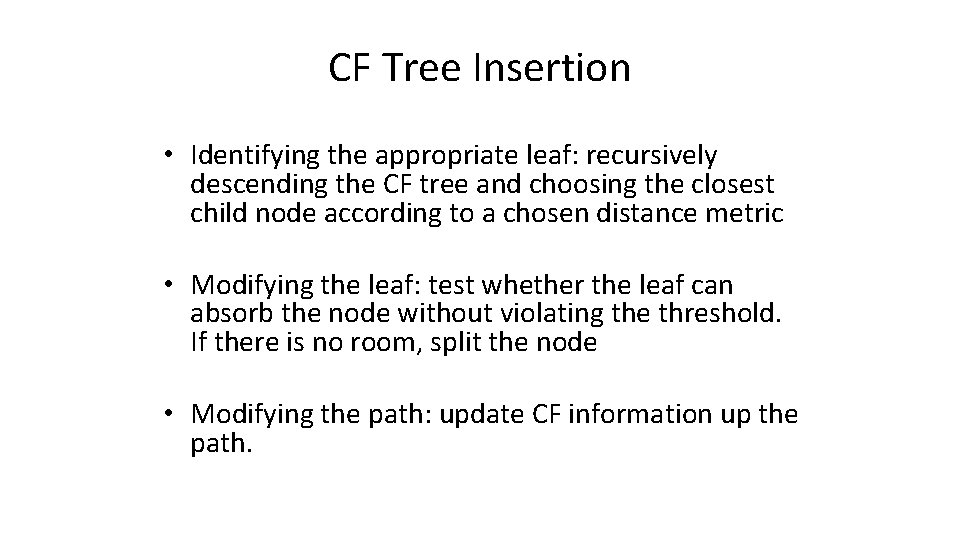
CF Tree Insertion • Identifying the appropriate leaf: recursively descending the CF tree and choosing the closest child node according to a chosen distance metric • Modifying the leaf: test whether the leaf can absorb the node without violating the threshold. If there is no room, split the node • Modifying the path: update CF information up the path. 42 of 28

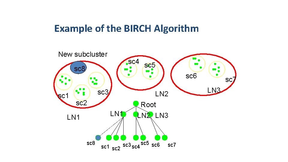
Example of the BIRCH Algorithm New subcluster sc 4 sc 5 sc 8 sc 1 sc 6 sc 3 sc 2 LN 1 sc 8 LN 2 Root LN 2 LN 3 sc 5 sc 6 sc 1 sc 2 sc 3 sc 4 sc 7 LN 3 sc 7 43 of 28

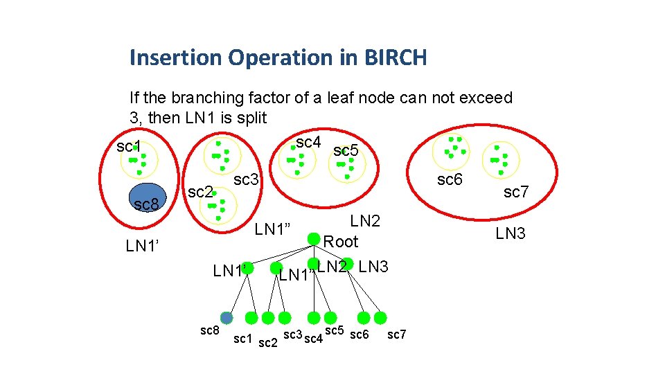
Insertion Operation in BIRCH If the branching factor of a leaf node can not exceed 3, then LN 1 is split sc 4 sc 5 sc 1 sc 8 sc 2 sc 3 sc 6 LN 2 Root LN 1” LN 2 LN 3 LN 1” LN 1’ sc 8 sc 5 sc 6 sc 1 sc 2 sc 3 sc 4 sc 7 LN 3

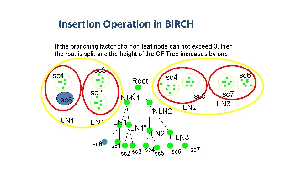
Insertion Operation in BIRCH If the branching factor of a non-leaf node can not exceed 3, then the root is split and the height of the CF Tree increases by one sc 1 sc 8 sc 3 Root sc 2 sc 5 LN 2 NLN 1 NLN 2 LN 1’ LN 1” LN 1’ sc 8 LN 1” sc 6 sc 4 LN 2 sc 1 sc 4 sc 2 sc 3 sc 5 sc 7 LN 3 sc 6 sc 7 19 of 28

Birch Clustering Algorithm (1) • Phase 1: Scan all data and build an initial in-memory CF tree. • Phase 2: condense into desirable length by building a smaller CF tree. • Phase 3: Global clustering • Phase 4: Cluster refining – this is optional, and requires more passes over the data to refine the results 20 of 28

Pros & Cons of BIRCH • Linear scalability – Good clustering with a single scan – Quality can be further improved by a few additional scans • Can handle only numeric data • Sensitive to the order of the data records

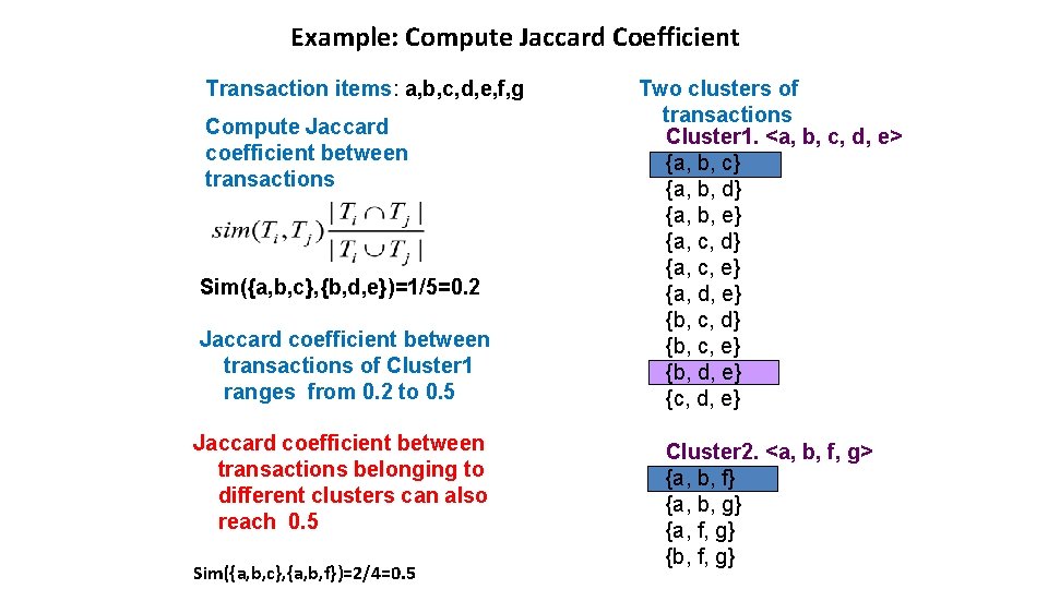
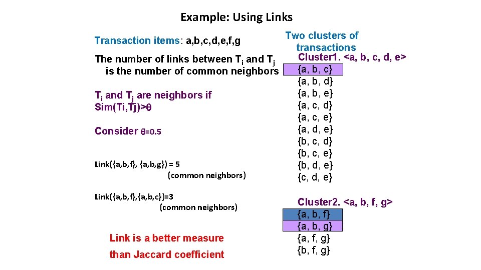
3. 3. 4 ROCK: for Categorical Data Experiments show that distance functions do not lead to high quality clusters when clustering categorical data Most clustering techniques assess the similarity between points to create clusters At each step, points that are similar are merged into a single cluster Localized approach prone to errors ROCK: used links instead of distances

Example: Compute Jaccard Coefficient Transaction items: a, b, c, d, e, f, g Compute Jaccard coefficient between transactions Sim({a, b, c}, {b, d, e})=1/5=0. 2 Jaccard coefficient between transactions of Cluster 1 ranges from 0. 2 to 0. 5 Jaccard coefficient between transactions belonging to different clusters can also reach 0. 5 Sim({a, b, c}, {a, b, f})=2/4=0. 5 Two clusters of transactions Cluster 1. <a, b, c, d, e> {a, b, c} {a, b, d} {a, b, e} {a, c, d} {a, c, e} {a, d, e} {b, c, d} {b, c, e} {b, d, e} {c, d, e} Cluster 2. <a, b, f, g> {a, b, f} {a, b, g} {a, f, g} {b, f, g}

Example: Using Links Two clusters of transactions Cluster 1. <a, b, c, d, e> The number of links between Ti and Tj {a, b, c} is the number of common neighbors {a, b, d} {a, b, e} Ti and Tj are neighbors if {a, c, d} Sim(Ti, Tj)> {a, c, e} {a, d, e} Consider =0. 5 {b, c, d} {b, c, e} Link({a, b, f}, {a, b, g}) = 5 {b, d, e} (common neighbors) {c, d, e} Transaction items: a, b, c, d, e, f, g Link({a, b, f}, {a, b, c})=3 (common neighbors) Link is a better measure than Jaccard coefficient Cluster 2. <a, b, f, g> {a, b, f} {a, b, g} {a, f, g} {b, f, g}

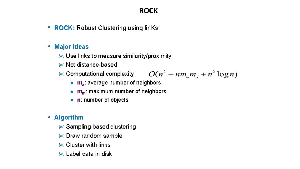
ROCK ROCK: Robust Clustering using lin. Ks Major Ideas " Use links to measure similarity/proximity " Not distance-based " Computational complexity ma: average number of neighbors mm: maximum number of neighbors n: number of objects Algorithm " Sampling-based clustering " Draw random sample " Cluster with links " Label data in disk

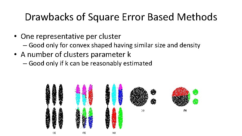
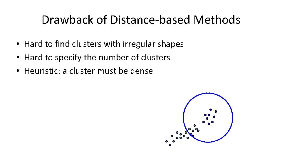
Drawbacks of Square Error Based Methods • One representative per cluster – Good only for convex shaped having similar size and density • A number of clusters parameter k – Good only if k can be reasonably estimated

Drawback of Distance-based Methods • Hard to find clusters with irregular shapes • Hard to specify the number of clusters • Heuristic: a cluster must be dense

DBSCAN – Density-Based Spatial Clustering of Applications with Noise Reference: M. Ester, H. P. Kriegel, J. Sander and Xu. A density-based algorithm for discovering clusters in large spatial databases, Aug 1996

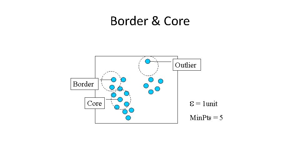
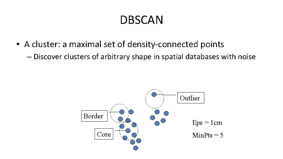
DBSCAN Density-based Clustering locates regions of high density that are separated from one another by regions of low density. – Density = number of points within a specified radius (Eps) • DBSCAN is a density-based algorithm. – A point is a core point if it has more than a specified number of points (Min. Pts) within Eps • These are points that are at the interior of a cluster – A border point has fewer than Min. Pts within Eps, but is in the neighborhood of a core point

DBSCAN – A noise point is any point that is not a core point or a border point. – Any two core points are close enough– within a distance Eps of one another – are put in the same cluster – Any border point that is close enough to a core point is put in the same cluster as the core point – Noise points are discarded

Border & Core Outlier Border Core = 1 unit Min. Pts = 5

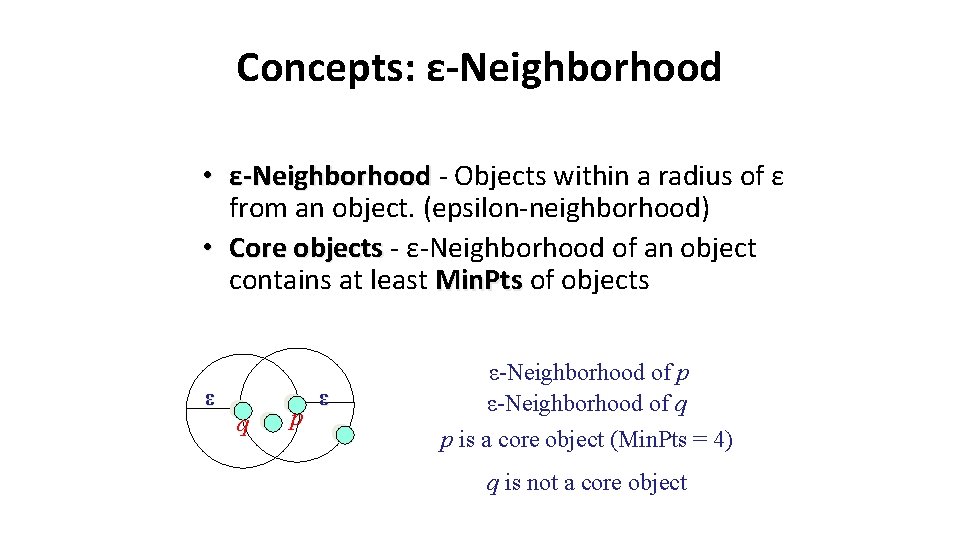
Concepts: ε-Neighborhood • ε-Neighborhood - Objects within a radius of ε from an object. (epsilon-neighborhood) • Core objects - ε-Neighborhood of an object contains at least Min. Pts of objects ε q p ε ε-Neighborhood of p ε-Neighborhood of q p is a core object (Min. Pts = 4) q is not a core object

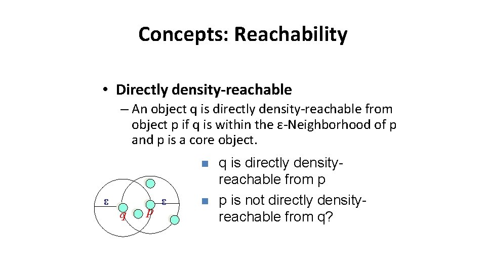
Concepts: Reachability • Directly density-reachable – An object q is directly density-reachable from object p if q is within the ε-Neighborhood of p and p is a core object. n ε q p ε n q is directly densityreachable from p p is not directly densityreachable from q?

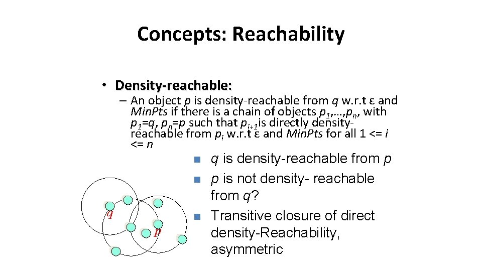
Concepts: Reachability • Density-reachable: – An object p is density-reachable from q w. r. t ε and Min. Pts if there is a chain of objects p 1, …, pn, with p 1=q, pn=p such that pi+1 is directly densityreachable from pi w. r. t ε and Min. Pts for all 1 <= i <= n n n q n p q is density-reachable from p p is not density- reachable from q? Transitive closure of direct density-Reachability, asymmetric

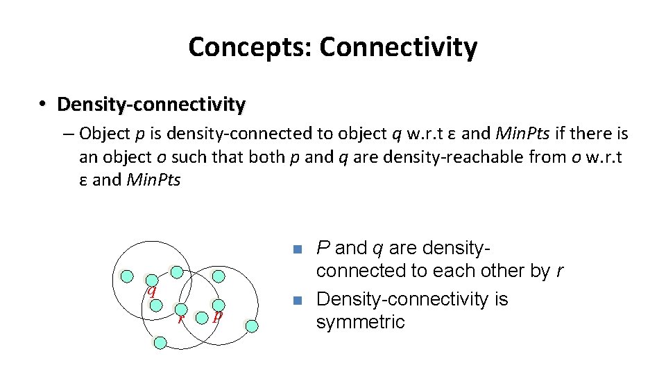
Concepts: Connectivity • Density-connectivity – Object p is density-connected to object q w. r. t ε and Min. Pts if there is an object o such that both p and q are density-reachable from o w. r. t ε and Min. Pts n q r p n P and q are densityconnected to each other by r Density-connectivity is symmetric

Concepts: cluster & noise • Cluster: Cluster a cluster C in a set of objects D w. r. t ε and Min. Pts is a non empty subset of D satisfying – Maximality: For all p, q if p C and if q is density-reachable from p w. r. t ε and Min. Pts, then also q C. – Connectivity: for all p, q C, p is density-connected to q w. r. t ε and Min. Pts in D. – Note: cluster contains core objects as well as border objects • Noise: objects which are not directly density-reachable from at least one core object.

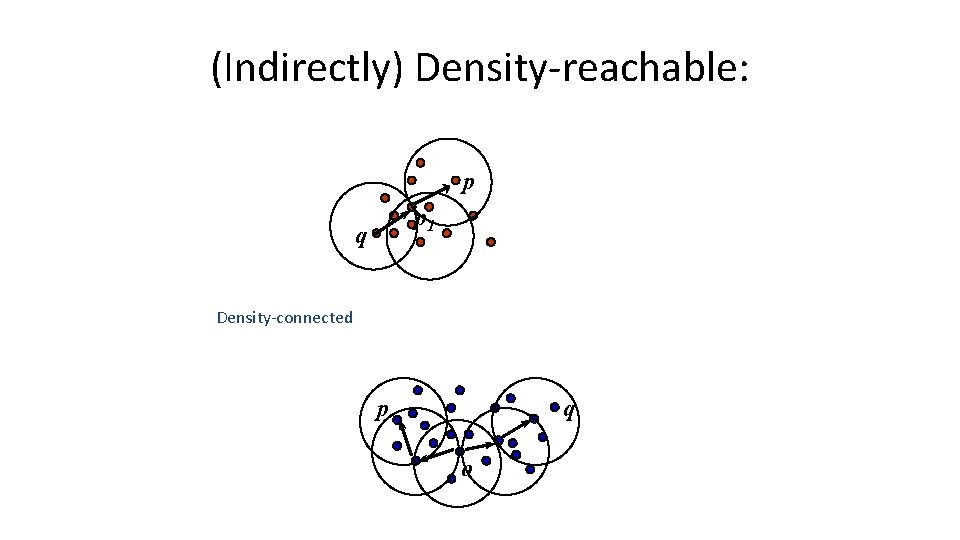
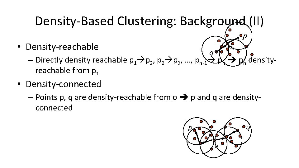
(Indirectly) Density-reachable: p p 1 q Density-connected p q o

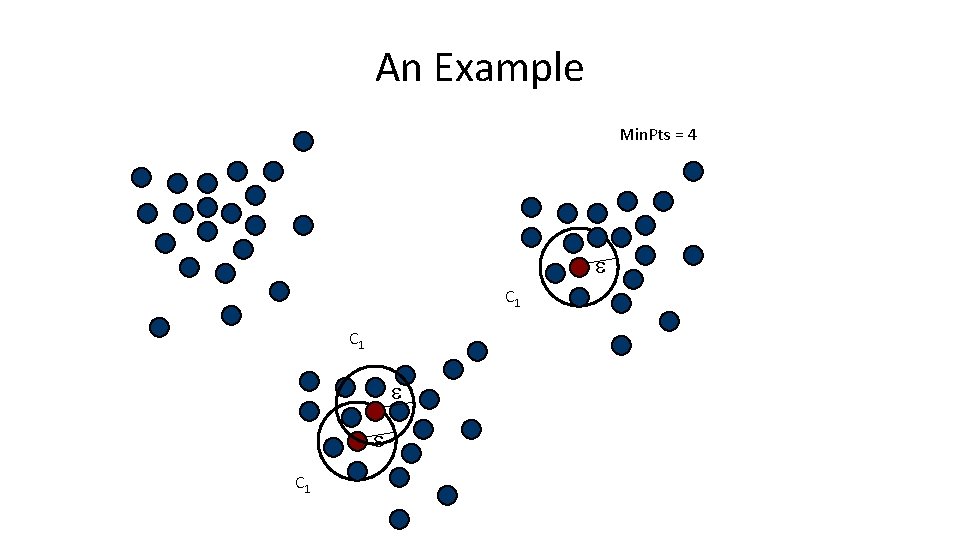
DBSCAN: The Algorithm – select a point p – Retrieve all points density-reachable from p wrt and Min. Pts. – If p is a core point, a cluster is formed. – If p is a border point, no points are density-reachable from p and DBSCAN visits the next point of the database. – Continue the process until all of the points have been processed.

An Example Min. Pts = 4 C 1 C 1

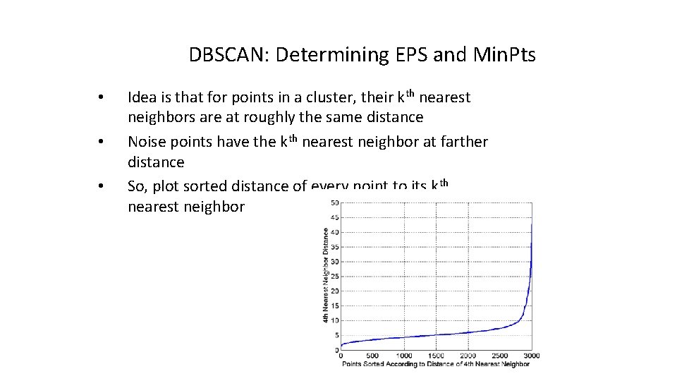
DBSCAN: Determining EPS and Min. Pts • • • Idea is that for points in a cluster, their kth nearest neighbors are at roughly the same distance Noise points have the kth nearest neighbor at farther distance So, plot sorted distance of every point to its kth nearest neighbor

DBSCAN: Determining EPS and Min. Pts • • • Distance from a point to its kth nearest neighbor=>kdist For points that belong to some clusters, the value of k -dist will be small if k is not larger than cluster size For points that are not in a cluster such as noise points, the k-dist will be relatively large Compute k-dist for all points for some k Sort them in increasing order and plot sorted values A sharp change at the value of k-dist that corresponds to suitable value of eps and the value of k as Min. Pts

DBSCAN: Determining EPS and Min. Pts • A sharp change at the value of k-dist that corresponds to suitable value of eps and the value of k as Min. Pts – • • Points for which k-dist is less than eps will be labeled as core points while other points will be labeled as noise or border points. If k is too large=> small clusters (of size less than k) are likely to be labeled as noise If k is too small=> Even a small number of closely spaced that are noise or outliers will be incorrectly labeled as clusters

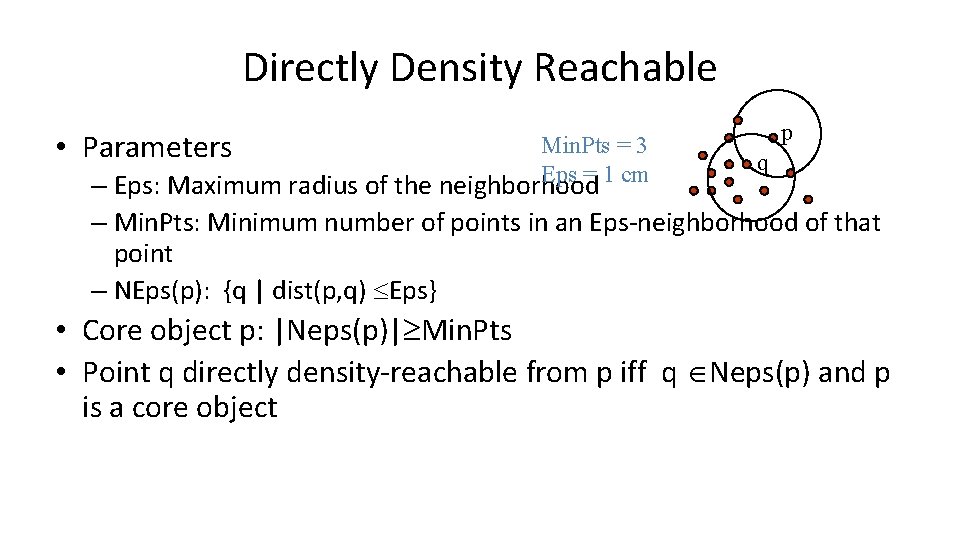
Directly Density Reachable • Parameters Min. Pts = 3 Eps = 1 cm p q – Eps: Maximum radius of the neighborhood – Min. Pts: Minimum number of points in an Eps-neighborhood of that point – NEps(p): {q | dist(p, q) Eps} • Core object p: |Neps(p)| Min. Pts • Point q directly density-reachable from p iff q Neps(p) and p is a core object

Density-Based Clustering: Background (II) p • Density-reachable p 1 q – Directly density reachable p 1 p 2, p 2 p 3, …, pn-1 pn densityreachable from p 1 • Density-connected – Points p, q are density-reachable from o p and q are densityconnected p q o

DBSCAN • A cluster: a maximal set of density-connected points – Discover clusters of arbitrary shape in spatial databases with noise Outlier Border Core Eps = 1 cm Min. Pts = 5

DBSCAN: the Algorithm • Arbitrary select a point p • Retrieve all points density-reachable from p wrt Eps and Min. Pts • If p is a core point, a cluster is formed • If p is a border point, no points are density-reachable from p and DBSCAN visits the next point of the database • Continue the process until all of the points have been processed

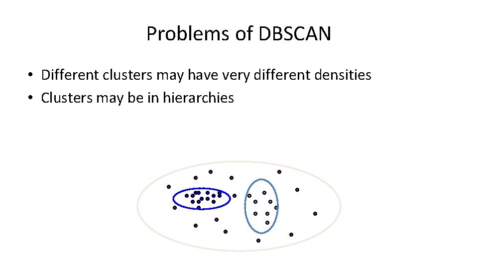
Problems of DBSCAN • Different clusters may have very different densities • Clusters may be in hierarchies