Classification CS 685 Special Topics in Data Mining

Classification CS 685: Special Topics in Data Mining Spring 2009 Jinze Liu The UNIVERSITY KENTUCKY CS 685 : Special Topics in Dataof Mining, UKY

Bayesian Classification: Why? • Probabilistic learning: Calculate explicit probabilities for hypothesis, among the most practical approaches to certain types of learning problems • Incremental: Each training example can incrementally increase/decrease the probability that a hypothesis is correct. Prior knowledge can be combined with observed data. • Probabilistic prediction: Predict multiple hypotheses, weighted by their probabilities • Standard: Even when Bayesian methods are computationally intractable, they can provide a standard of optimal decision making against which other methods can be measured CS 685 : Special Topics in Data Mining, UKY

Bayesian Theorem: Basics • Let X be a data sample whose class label is unknown • Let H be a hypothesis that X belongs to class C • For classification problems, determine P(H/X): the probability that the hypothesis holds given the observed data sample X • P(H): prior probability of hypothesis H (i. e. the initial probability before we observe any data, reflects the background knowledge) • P(X): probability that sample data is observed • P(X|H) : probability of observing the sample X, given that the hypothesis holds CS 685 : Special Topics in Data Mining, UKY

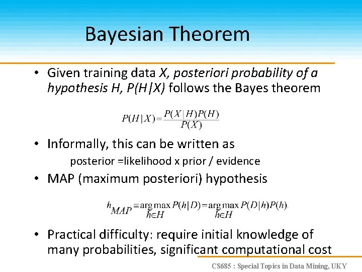
Bayesian Theorem • Given training data X, posteriori probability of a hypothesis H, P(H|X) follows the Bayes theorem • Informally, this can be written as posterior =likelihood x prior / evidence • MAP (maximum posteriori) hypothesis • Practical difficulty: require initial knowledge of many probabilities, significant computational cost CS 685 : Special Topics in Data Mining, UKY

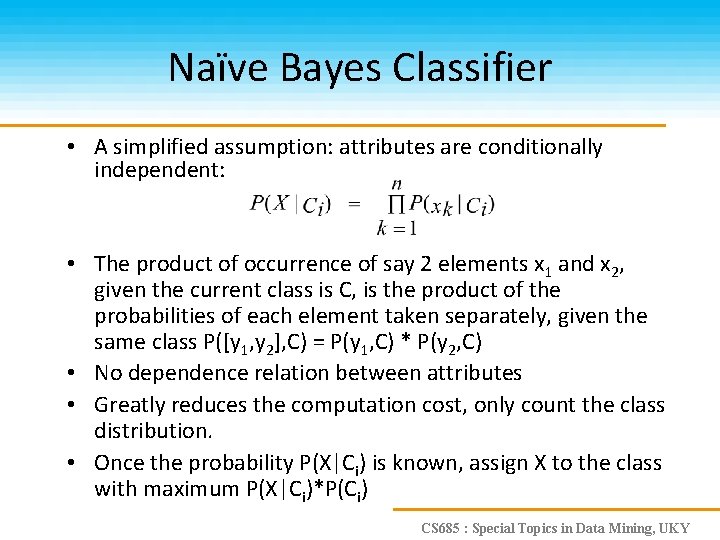
Naïve Bayes Classifier • A simplified assumption: attributes are conditionally independent: • The product of occurrence of say 2 elements x 1 and x 2, given the current class is C, is the product of the probabilities of each element taken separately, given the same class P([y 1, y 2], C) = P(y 1, C) * P(y 2, C) • No dependence relation between attributes • Greatly reduces the computation cost, only count the class distribution. • Once the probability P(X|Ci) is known, assign X to the class with maximum P(X|Ci)*P(Ci) CS 685 : Special Topics in Data Mining, UKY

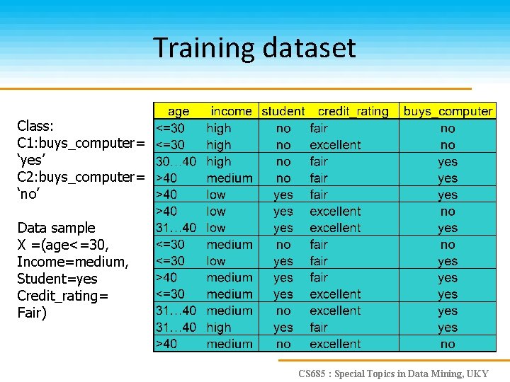
Training dataset Class: C 1: buys_computer= ‘yes’ C 2: buys_computer= ‘no’ Data sample X =(age<=30, Income=medium, Student=yes Credit_rating= Fair) CS 685 : Special Topics in Data Mining, UKY

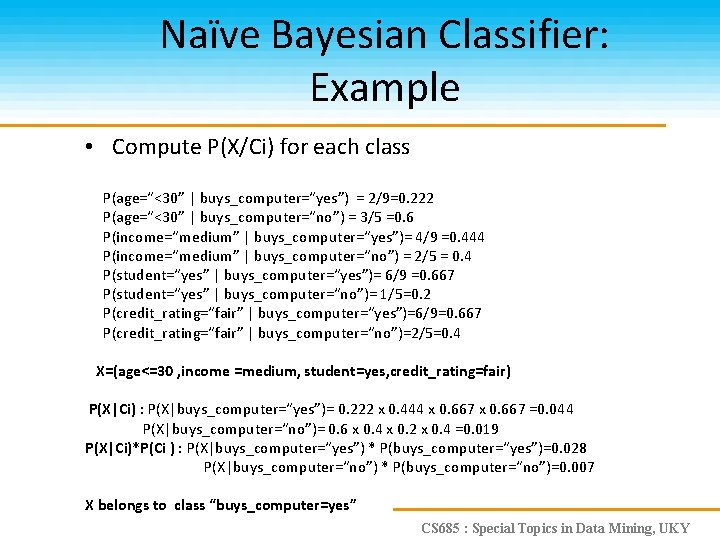
Naïve Bayesian Classifier: Example • Compute P(X/Ci) for each class P(age=“<30” | buys_computer=“yes”) = 2/9=0. 222 P(age=“<30” | buys_computer=“no”) = 3/5 =0. 6 P(income=“medium” | buys_computer=“yes”)= 4/9 =0. 444 P(income=“medium” | buys_computer=“no”) = 2/5 = 0. 4 P(student=“yes” | buys_computer=“yes”)= 6/9 =0. 667 P(student=“yes” | buys_computer=“no”)= 1/5=0. 2 P(credit_rating=“fair” | buys_computer=“yes”)=6/9=0. 667 P(credit_rating=“fair” | buys_computer=“no”)=2/5=0. 4 X=(age<=30 , income =medium, student=yes, credit_rating=fair) P(X|Ci) : P(X|buys_computer=“yes”)= 0. 222 x 0. 444 x 0. 667 =0. 044 P(X|buys_computer=“no”)= 0. 6 x 0. 4 x 0. 2 x 0. 4 =0. 019 P(X|Ci)*P(Ci ) : P(X|buys_computer=“yes”) * P(buys_computer=“yes”)=0. 028 P(X|buys_computer=“no”) * P(buys_computer=“no”)=0. 007 X belongs to class “buys_computer=yes” CS 685 : Special Topics in Data Mining, UKY

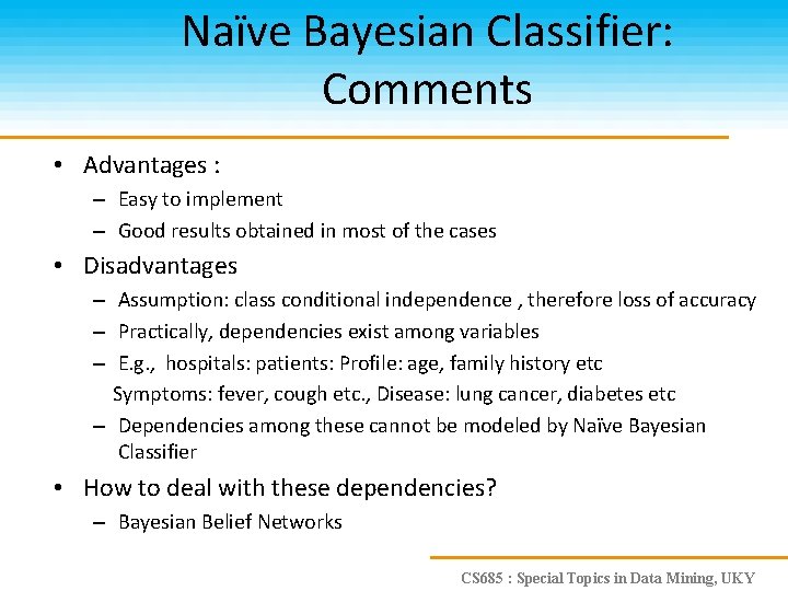
Naïve Bayesian Classifier: Comments • Advantages : – Easy to implement – Good results obtained in most of the cases • Disadvantages – Assumption: class conditional independence , therefore loss of accuracy – Practically, dependencies exist among variables – E. g. , hospitals: patients: Profile: age, family history etc Symptoms: fever, cough etc. , Disease: lung cancer, diabetes etc – Dependencies among these cannot be modeled by Naïve Bayesian Classifier • How to deal with these dependencies? – Bayesian Belief Networks CS 685 : Special Topics in Data Mining, UKY

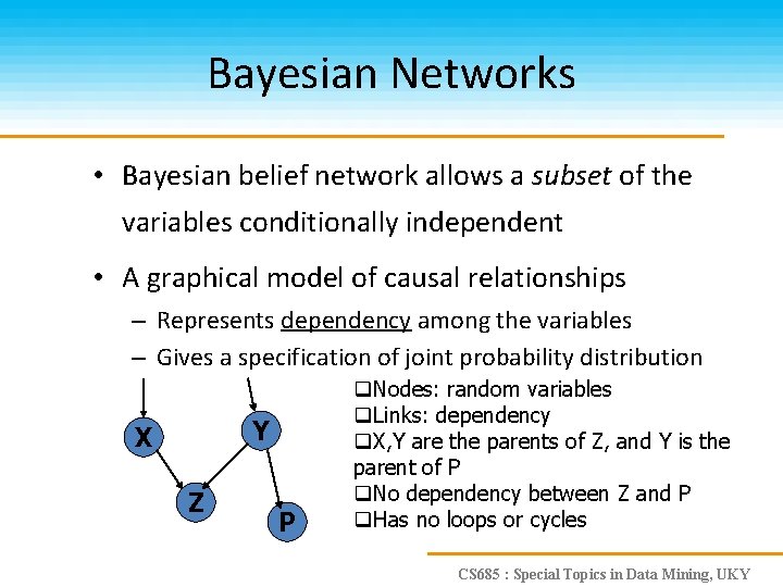
Bayesian Networks • Bayesian belief network allows a subset of the variables conditionally independent • A graphical model of causal relationships – Represents dependency among the variables – Gives a specification of joint probability distribution Y X Z P q. Nodes: random variables q. Links: dependency q. X, Y are the parents of Z, and Y is the parent of P q. No dependency between Z and P q. Has no loops or cycles CS 685 : Special Topics in Data Mining, UKY

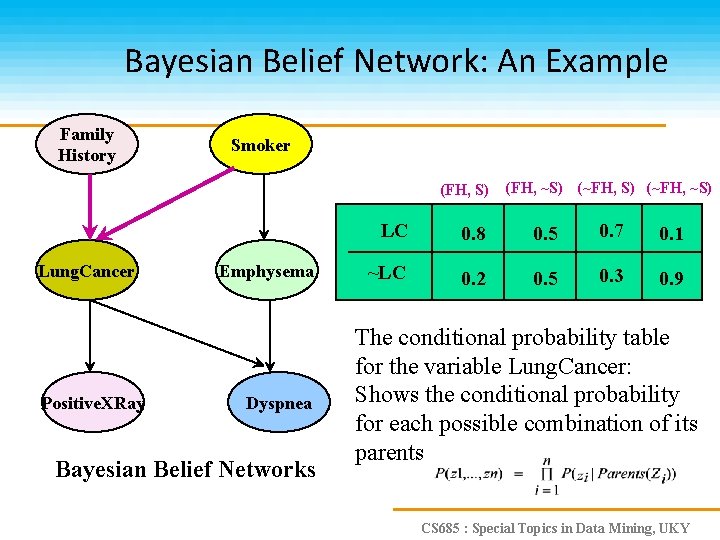
Bayesian Belief Network: An Example Family History Smoker (FH, S) Lung. Cancer Positive. XRay Emphysema Dyspnea Bayesian Belief Networks (FH, ~S) (~FH, ~S) LC 0. 8 0. 5 0. 7 0. 1 ~LC 0. 2 0. 5 0. 3 0. 9 The conditional probability table for the variable Lung. Cancer: Shows the conditional probability for each possible combination of its parents CS 685 : Special Topics in Data Mining, UKY

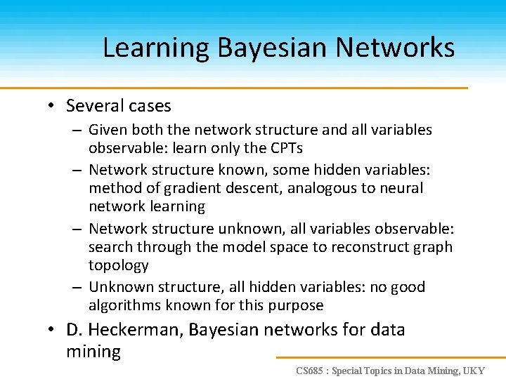
Learning Bayesian Networks • Several cases – Given both the network structure and all variables observable: learn only the CPTs – Network structure known, some hidden variables: method of gradient descent, analogous to neural network learning – Network structure unknown, all variables observable: search through the model space to reconstruct graph topology – Unknown structure, all hidden variables: no good algorithms known for this purpose • D. Heckerman, Bayesian networks for data mining CS 685 : Special Topics in Data Mining, UKY

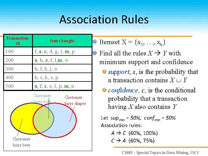
Association Rules Transactionid Items bought 100 f, a, c, d, g, I, m, p 200 a, b, c, f, l, m, o 300 b, f, h, j, o 400 b, c, k, s, p 500 a, f, c, e, l, p, m, n Customer buys both Customer buys beer Customer buys diaper Itemset X = {x 1, …, xk} Find all the rules X Y with minimum support and confidence support, s, is the probability that a transaction contains X Y confidence, c, is the conditional probability that a transaction having X also contains Y Let supmin = 50%, confmin = 50% Association rules: A C (60%, 100%) C A (60%, 75%) CS 685 : Special Topics in Data Mining, UKY

Classification based on Association • Classification rule mining versus Association rule mining • Aim – A small set of rules as classifier – All rules according to minsup and minconf • Syntax – X y – X Y CS 685 : Special Topics in Data Mining, UKY

Why & How to Integrate • Both classification rule mining and association rule mining are indispensable to practical applications. • The integration is done by focusing on a special subset of association rules whose right-hand-side are restricted to the classification class attribute. – CARs: class association rules CS 685 : Special Topics in Data Mining, UKY

CBA: Three Steps • Discretize continuous attributes, if any • Generate all class association rules (CARs) • Build a classifier based on the generated CARs. CS 685 : Special Topics in Data Mining, UKY

Our Objectives • To generate the complete set of CARs that satisfy the user-specified minimum support (minsup) and minimum confidence (minconf) constraints. • To build a classifier from the CARs. CS 685 : Special Topics in Data Mining, UKY

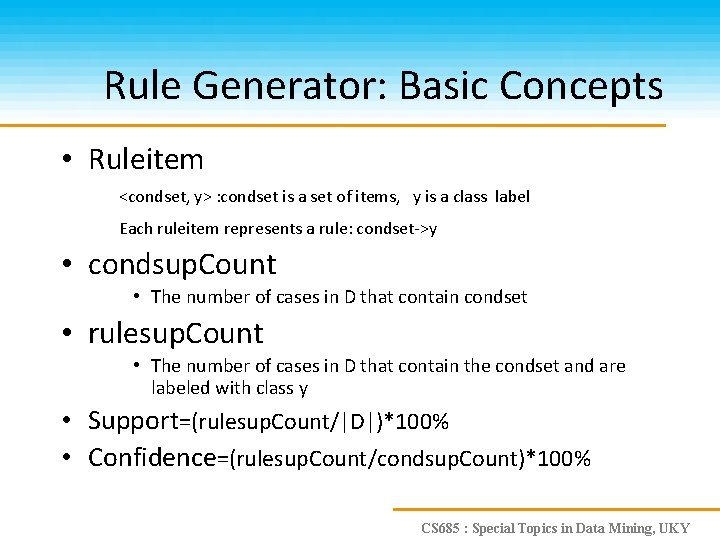
Rule Generator: Basic Concepts • Ruleitem <condset, y> : condset is a set of items, y is a class label Each ruleitem represents a rule: condset->y • condsup. Count • The number of cases in D that contain condset • rulesup. Count • The number of cases in D that contain the condset and are labeled with class y • Support=(rulesup. Count/|D|)*100% • Confidence=(rulesup. Count/condsup. Count)*100% CS 685 : Special Topics in Data Mining, UKY

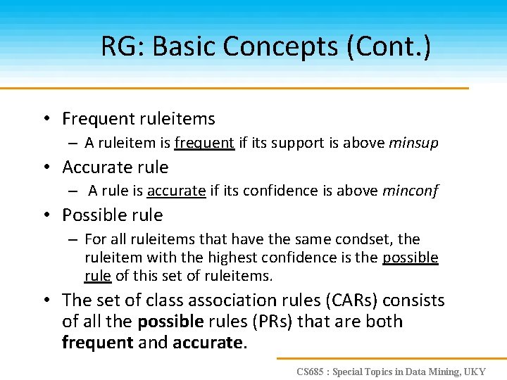
RG: Basic Concepts (Cont. ) • Frequent ruleitems – A ruleitem is frequent if its support is above minsup • Accurate rule – A rule is accurate if its confidence is above minconf • Possible rule – For all ruleitems that have the same condset, the ruleitem with the highest confidence is the possible rule of this set of ruleitems. • The set of class association rules (CARs) consists of all the possible rules (PRs) that are both frequent and accurate. CS 685 : Special Topics in Data Mining, UKY

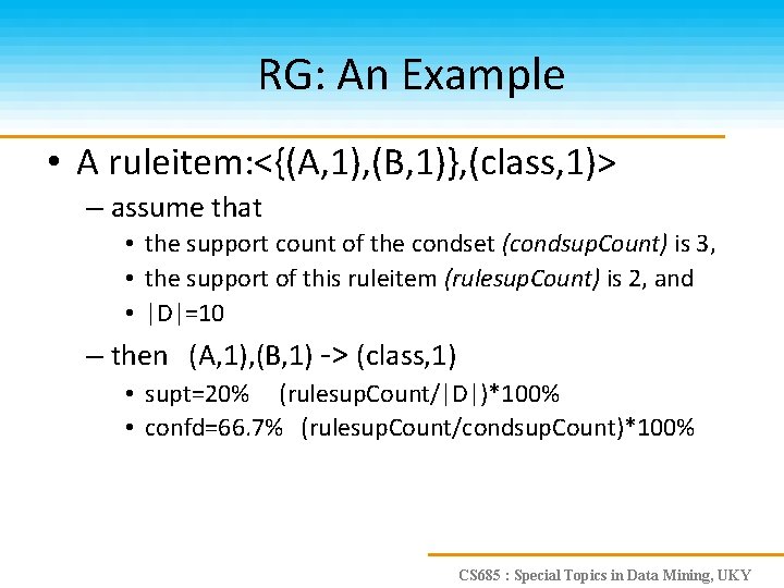
RG: An Example • A ruleitem: <{(A, 1), (B, 1)}, (class, 1)> – assume that • the support count of the condset (condsup. Count) is 3, • the support of this ruleitem (rulesup. Count) is 2, and • |D|=10 – then (A, 1), (B, 1) -> (class, 1) • supt=20% (rulesup. Count/|D|)*100% • confd=66. 7% (rulesup. Count/condsup. Count)*100% CS 685 : Special Topics in Data Mining, UKY

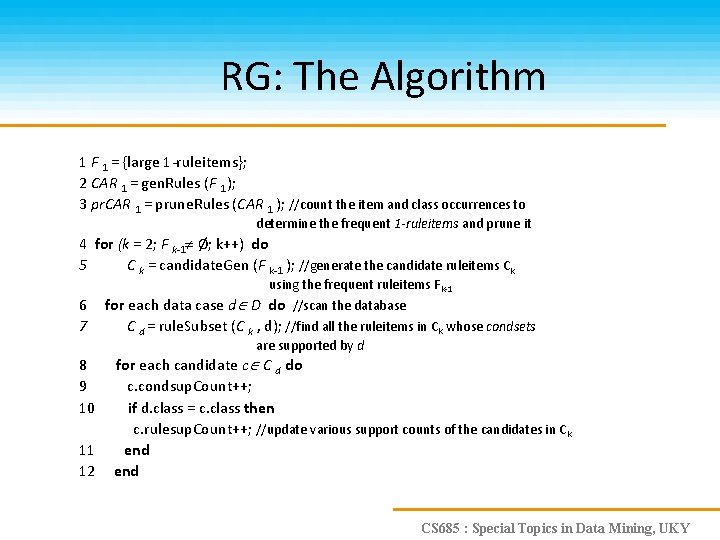
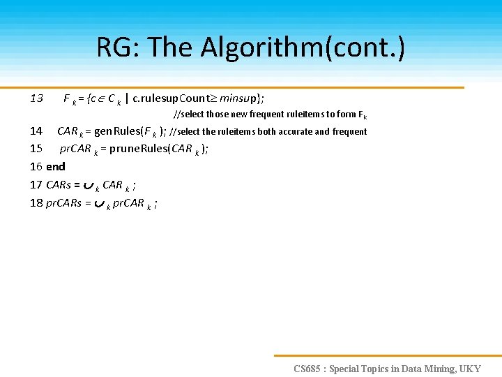
RG: The Algorithm 1 F 1 = {large 1 -ruleitems}; 2 CAR 1 = gen. Rules (F 1 ); 3 pr. CAR 1 = prune. Rules (CAR 1 ); //count the item and class occurrences to determine the frequent 1 -ruleitems and prune it 4 for (k = 2; F k-1 Ø; k++) do 5 C k = candidate. Gen (F k-1 ); //generate the candidate ruleitems Ck 6 7 using the frequent ruleitems Fk-1 for each data case d D do //scan the database C d = rule. Subset (C k , d); //find all the ruleitems in Ck whose condsets are supported by d 8 9 10 11 12 for each candidate c C d do c. condsup. Count++; if d. class = c. class then c. rulesup. Count++; //update various support counts of the candidates in Ck end CS 685 : Special Topics in Data Mining, UKY

RG: The Algorithm(cont. ) 13 F k = {c C k | c. rulesup. Count minsup}; //select those new frequent ruleitems to form Fk 14 CAR k = gen. Rules(F k ); //select the ruleitems both accurate and frequent 15 pr. CAR k = prune. Rules(CAR k ); 16 end 17 CARs = k CAR k ; 18 pr. CARs = k pr. CAR k ; CS 685 : Special Topics in Data Mining, UKY

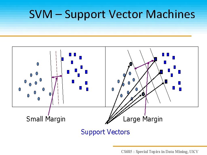
SVM – Support Vector Machines Small Margin Large Margin Support Vectors CS 685 : Special Topics in Data Mining, UKY

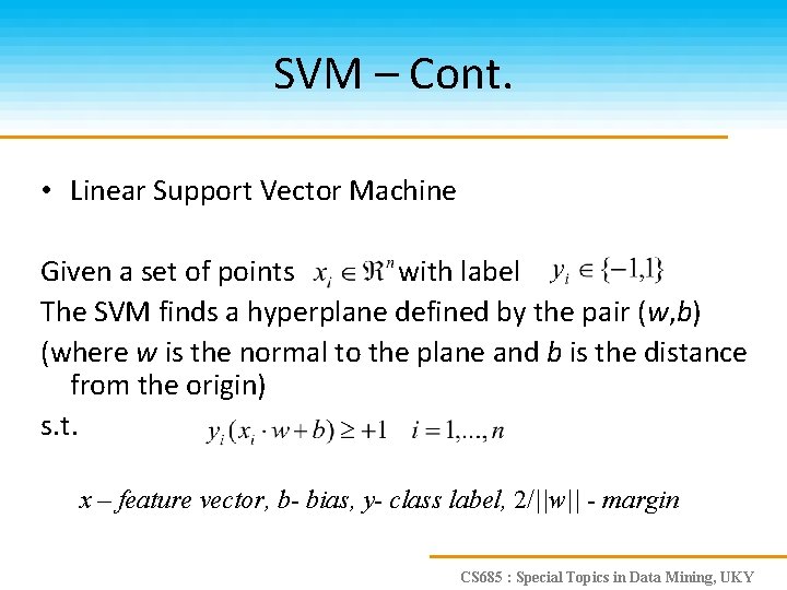
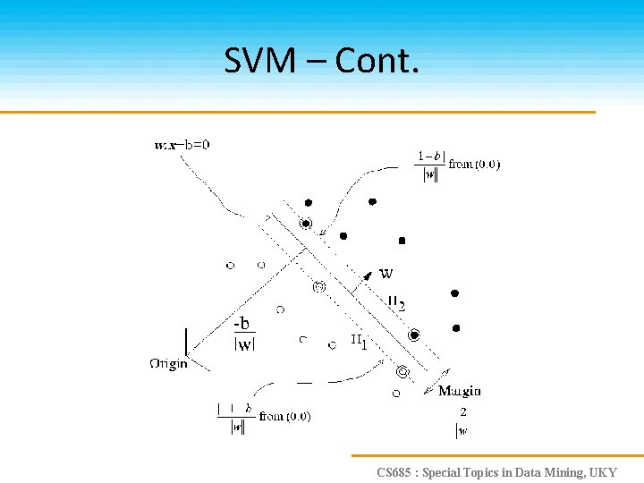
SVM – Cont. • Linear Support Vector Machine Given a set of points with label The SVM finds a hyperplane defined by the pair (w, b) (where w is the normal to the plane and b is the distance from the origin) s. t. x – feature vector, b- bias, y- class label, 2/||w|| - margin CS 685 : Special Topics in Data Mining, UKY

SVM – Cont. CS 685 : Special Topics in Data Mining, UKY

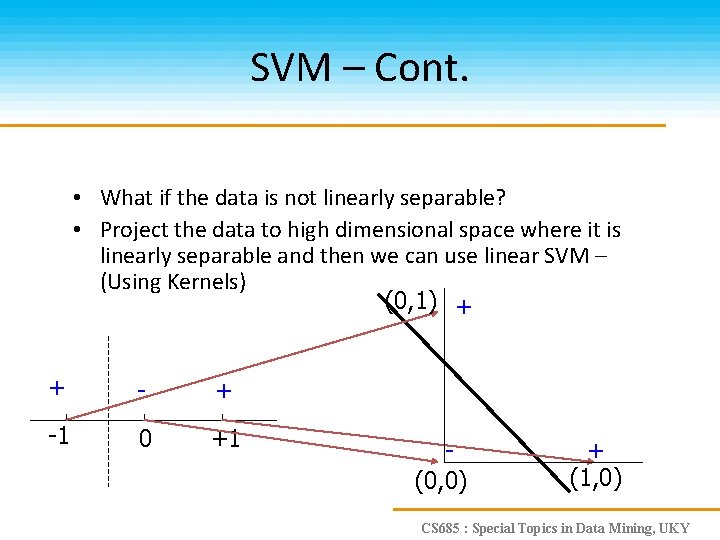
SVM – Cont. • What if the data is not linearly separable? • Project the data to high dimensional space where it is linearly separable and then we can use linear SVM – (Using Kernels) (0, 1) + + -1 0 +1 (0, 0) + (1, 0) CS 685 : Special Topics in Data Mining, UKY

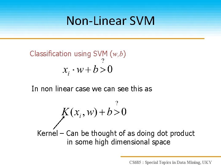
Non-Linear SVM Classification using SVM (w, b) In non linear case we can see this as Kernel – Can be thought of as doing dot product in some high dimensional space CS 685 : Special Topics in Data Mining, UKY

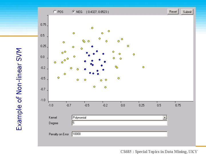
Example of Non-linear SVM CS 685 : Special Topics in Data Mining, UKY

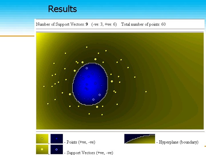
Results CS 685 : Special Topics in Data Mining, UKY

SVM Related Links • http: //svm. dcs. rhbnc. ac. uk/ • http: //www. kernel-machines. org/ • C. J. C. Burges. A Tutorial on Support Vector Machines for Pattern Recognition. Knowledge Discovery and Data Mining, 2(2), 1998. • SVMlight – Software (in C) http: //ais. gmd. de/~thorsten/svm_light • BOOK: An Introduction to Support Vector Machines N. Cristianini and J. Shawe-Taylor Cambridge University Press CS 685 : Special Topics in Data Mining, UKY