Clustering CS 685 Special Topics in Data Mining

Clustering CS 685: Special Topics in Data Mining Jinze Liu The UNIVERSITY KENTUCKY CS 685 : Special Topics in Dataof Mining, UKY

Outline • • What is clustering Partitioning methods Hierarchical methods Density-based methods Grid-based methods Model-based clustering methods Outlier analysis CS 685 : Special Topics in Data Mining, UKY

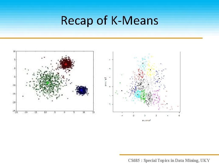
Recap of K-Means CS 685 : Special Topics in Data Mining, UKY

Family Tree CS 685 : Special Topics in Data Mining, UKY

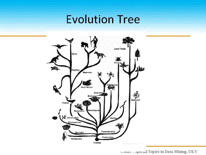
Evolution Tree CS 685 : Special Topics in Data Mining, UKY

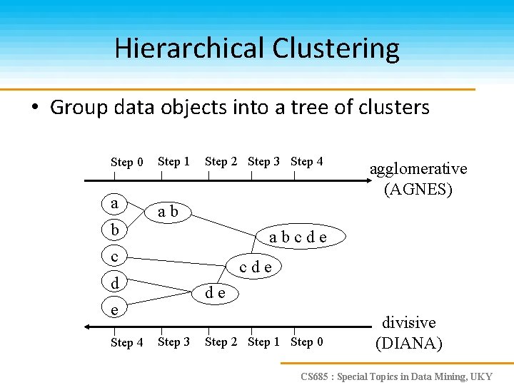
Hierarchical Clustering • Group data objects into a tree of clusters Step 0 a b Step 1 Step 2 Step 3 Step 4 ab abcde c cde d de e Step 4 agglomerative (AGNES) Step 3 Step 2 Step 1 Step 0 divisive (DIANA) CS 685 : Special Topics in Data Mining, UKY

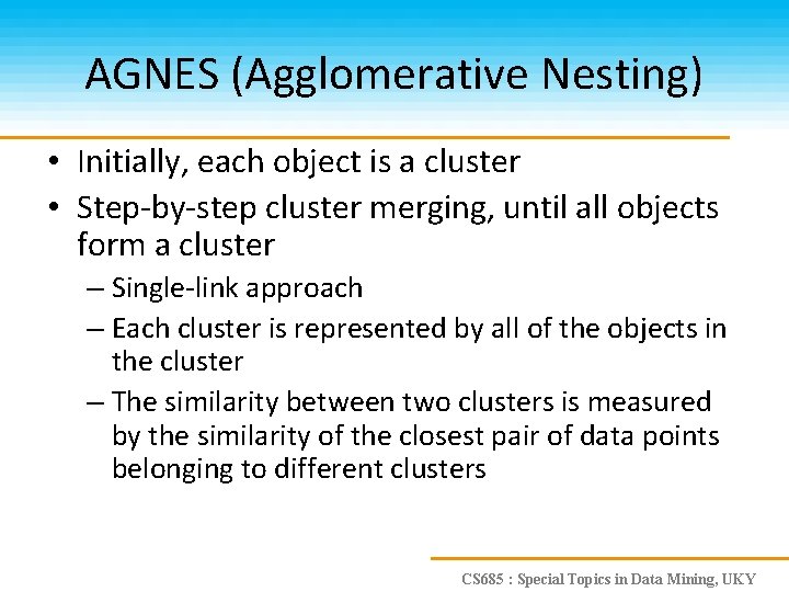
AGNES (Agglomerative Nesting) • Initially, each object is a cluster • Step-by-step cluster merging, until all objects form a cluster – Single-link approach – Each cluster is represented by all of the objects in the cluster – The similarity between two clusters is measured by the similarity of the closest pair of data points belonging to different clusters CS 685 : Special Topics in Data Mining, UKY

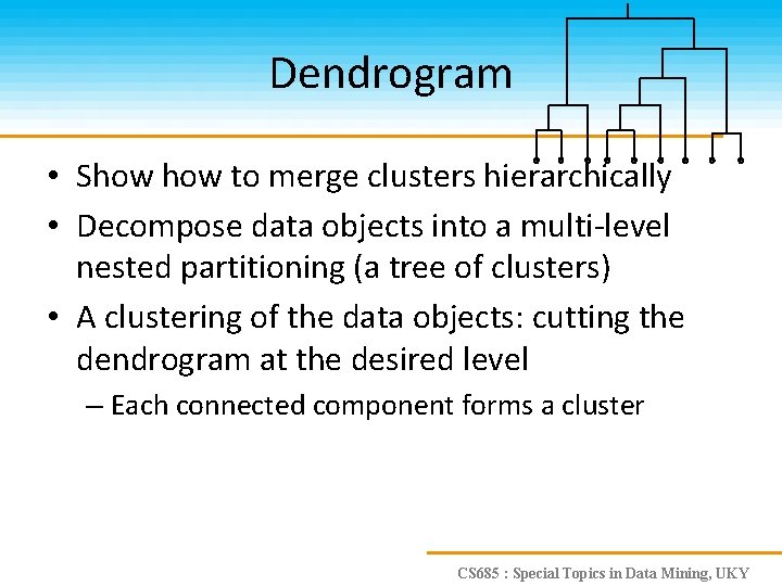
Dendrogram • Show to merge clusters hierarchically • Decompose data objects into a multi-level nested partitioning (a tree of clusters) • A clustering of the data objects: cutting the dendrogram at the desired level – Each connected component forms a cluster CS 685 : Special Topics in Data Mining, UKY

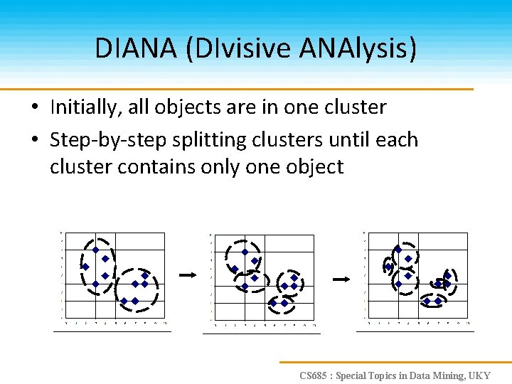
DIANA (DIvisive ANAlysis) • Initially, all objects are in one cluster • Step-by-step splitting clusters until each cluster contains only one object CS 685 : Special Topics in Data Mining, UKY

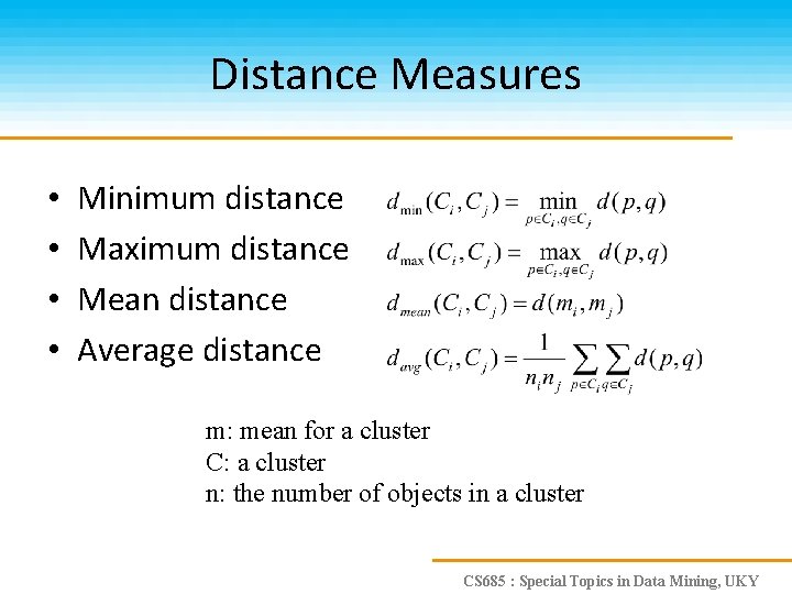
Distance Measures • • Minimum distance Maximum distance Mean distance Average distance m: mean for a cluster C: a cluster n: the number of objects in a cluster CS 685 : Special Topics in Data Mining, UKY

Challenges of Hierarchical Clustering Methods • Hard to choose merge/split points – Never undo merging/splitting – Merging/splitting decisions are critical • Do not scale well: O(n 3) • What is the bottleneck when the data cannot fit in memory? • Integrating hierarchical clustering with other techniques – BIRCH, CURE, CHAMELEON, ROCK CS 685 : Special Topics in Data Mining, UKY

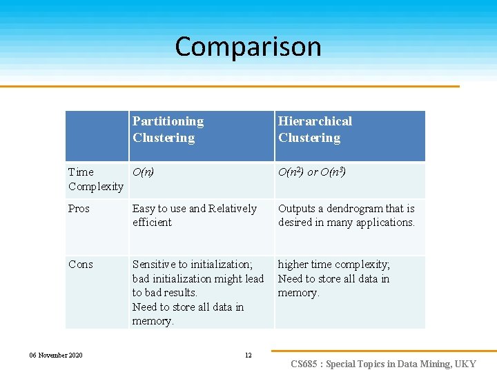
Comparison Partitioning Clustering Hierarchical Clustering Time O(n) Complexity O(n 2) or O(n 3) Pros Easy to use and Relatively efficient Outputs a dendrogram that is desired in many applications. Cons Sensitive to initialization; bad initialization might lead to bad results. Need to store all data in memory. higher time complexity; Need to store all data in memory. 06 November 2020 12 CS 685 : Special Topics in Data Mining, UKY

BIRCH Balanced Iterative Reducing and Clustering using Hierarchies The UNIVERSITY KENTUCKY CS 685 : Special Topics in Dataof Mining, UKY

Introduction to BIRCH • Designed for very large data sets – – Time and memory are limited Incremental and dynamic clustering of incoming objects Only one scan of data is necessary Does not need the whole data set in advance • Two key phases: – Scans the database to build an in-memory tree – Applies clustering algorithm to cluster the leaf nodes 06 November 2020 14 CS 685 : Special Topics in Data Mining, UKY

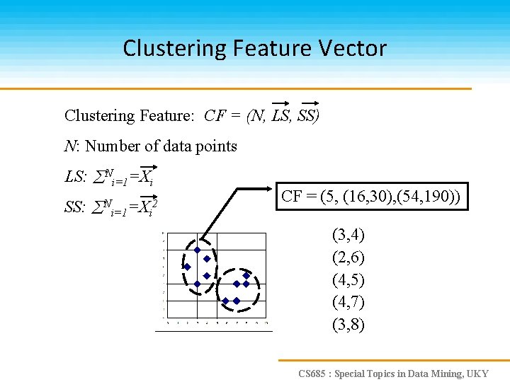
Clustering Feature Vector Clustering Feature: CF = (N, LS, SS) N: Number of data points LS: Ni=1=Xi SS: N 2 i=1=Xi CF = (5, (16, 30), (54, 190)) (3, 4) (2, 6) (4, 5) (4, 7) (3, 8) CS 685 : Special Topics in Data Mining, UKY

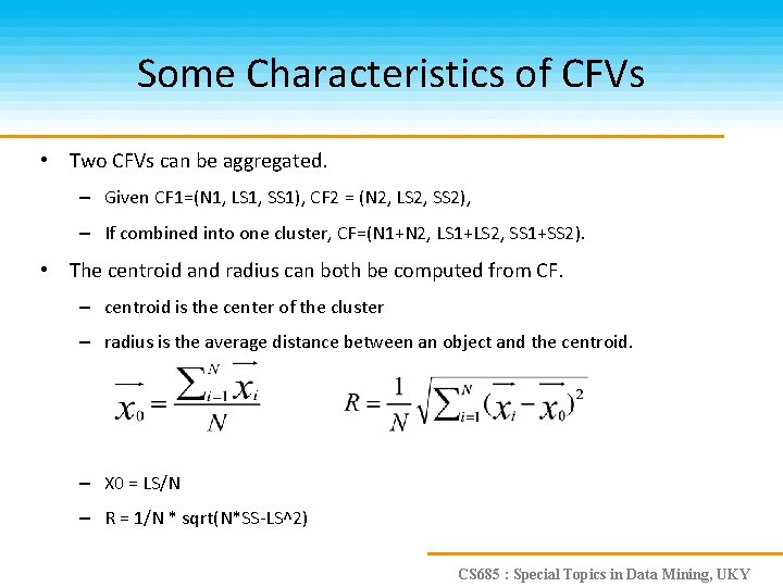
Some Characteristics of CFVs • Two CFVs can be aggregated. – Given CF 1=(N 1, LS 1, SS 1), CF 2 = (N 2, LS 2, SS 2), – If combined into one cluster, CF=(N 1+N 2, LS 1+LS 2, SS 1+SS 2). • The centroid and radius can both be computed from CF. – centroid is the center of the cluster – radius is the average distance between an object and the centroid. – X 0 = LS/N – R = 1/N * sqrt(N*SS-LS^2) CS 685 : Special Topics in Data Mining, UKY

Clustering Feature • Clustering feature: – Summarize the statistics for a subcluster • the 0 th, 1 st and 2 nd moments of the subcluster – Register crucial measurements for computing cluster and utilize storage efficiently CS 685 : Special Topics in Data Mining, UKY

CF-tree in BIRCH • A CF tree: a height-balanced tree storing the clustering features for a hierarchical clustering – A nonleaf node in a tree has descendants or “children” – The nonleaf nodes store sums of the CFs of children CS 685 : Special Topics in Data Mining, UKY

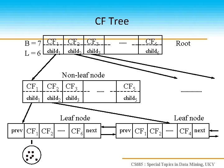
CF Tree B = 7 CF 1 CF 2 CF 3 L = 6 child 1 child 2 child 3 CF 6 child 6 CF 1 Non-leaf node CF 2 CF 3 CF 5 child 1 child 2 child 3 child 5 Leaf node prev CF 1 CF 2 CF 6 next Root Leaf node prev CF 1 CF 2 CF 4 next CS 685 : Special Topics in Data Mining, UKY

Parameters of A CF-tree • Branching factor: the maximum number of children • Threshold: max diameter of sub-clusters stored at the leaf nodes CS 685 : Special Topics in Data Mining, UKY

CF Tree Insertion • Identifying the appropriate leaf: recursively descending the CF tree and choosing the closest child node according to a chosen distance metric • Modifying the leaf: test whether the leaf can absorb the node without violating the threshold. If there is no room, split the node • Modifying the path: update CF information up the path. 22 of 28 CS 685 : Special Topics in Data Mining, UKY

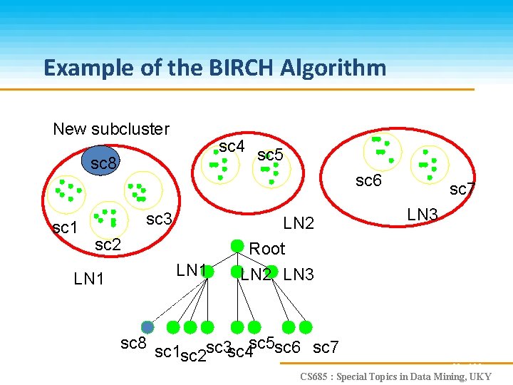
Example of the BIRCH Algorithm New subcluster sc 4 sc 5 sc 8 sc 1 sc 6 sc 3 sc 2 LN 1 LN 2 Root LN 2 LN 3 sc 8 sc 1 sc 3 sc 4 sc 5 sc 6 sc 7 sc 2 sc 7 LN 3 23 of 28 CS 685 : Special Topics in Data Mining, UKY

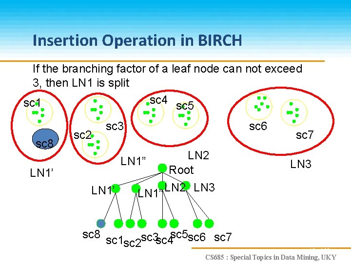
Insertion Operation in BIRCH If the branching factor of a leaf node can not exceed 3, then LN 1 is split sc 4 sc 5 sc 1 sc 8 sc 2 sc 3 sc 6 LN 2 Root LN 1” LN 2 LN 3 LN 1” LN 1’ sc 8 sc 1 sc 3 sc 4 sc 5 sc 6 sc 7 sc 2 sc 7 LN 3 19 of 28 CS 685 : Special Topics in Data Mining, UKY

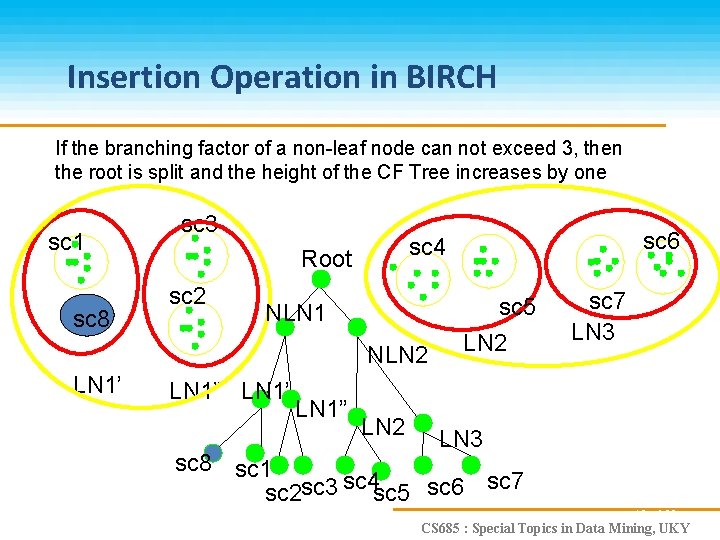
Insertion Operation in BIRCH If the branching factor of a non-leaf node can not exceed 3, then the root is split and the height of the CF Tree increases by one sc 1 sc 8 sc 3 Root sc 2 NLN 1 NLN 2 LN 1’ LN 1” sc 6 sc 4 LN 2 sc 5 LN 2 sc 7 LN 3 sc 8 sc 1 sc 2 sc 3 sc 4 sc 5 sc 6 sc 7 19 of 28 CS 685 : Special Topics in Data Mining, UKY

Birch Clustering Algorithm (1) • Phase 1: Scan all data and build an initial inmemory CF tree. • Phase 2: condense into desirable length by building a smaller CF tree. • Phase 3: Global clustering • Phase 4: Cluster refining – this is optional, and requires more passes over the data to refine the results 20 of 28 CS 685 : Special Topics in Data Mining, UKY

Pros & Cons of BIRCH • Linear scalability – Good clustering with a single scan – Quality can be further improved by a few additional scans • Can handle only numeric data • Sensitive to the order of the data records CS 685 : Special Topics in Data Mining, UKY

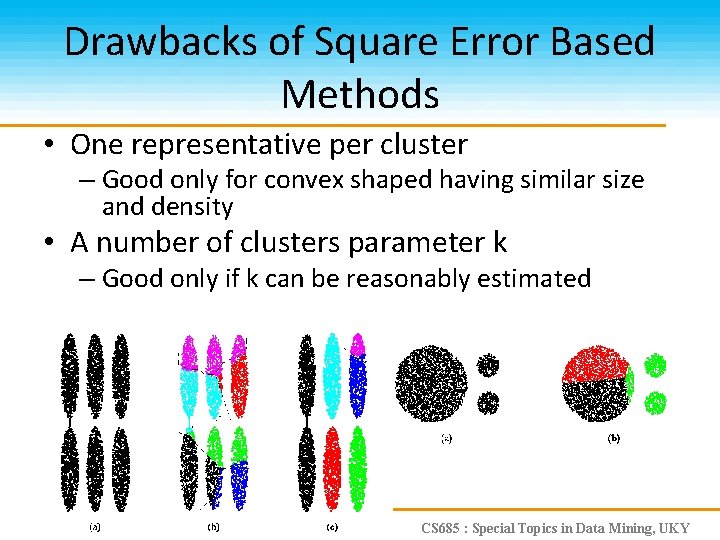
Drawbacks of Square Error Based Methods • One representative per cluster – Good only for convex shaped having similar size and density • A number of clusters parameter k – Good only if k can be reasonably estimated CS 685 : Special Topics in Data Mining, UKY

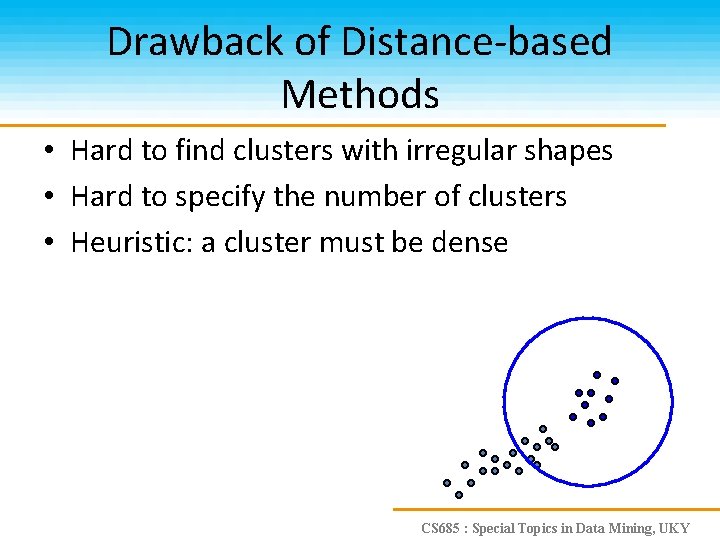
Drawback of Distance-based Methods • Hard to find clusters with irregular shapes • Hard to specify the number of clusters • Heuristic: a cluster must be dense CS 685 : Special Topics in Data Mining, UKY

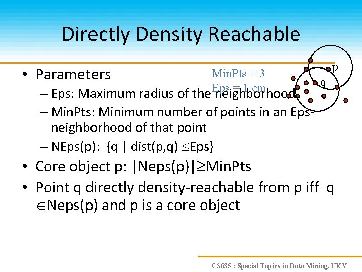
Directly Density Reachable • Parameters Min. Pts = 3 Eps = 1 cm – Eps: Maximum radius of the neighborhood – Min. Pts: Minimum number of points in an Epsneighborhood of that point – NEps(p): {q | dist(p, q) Eps} p q • Core object p: |Neps(p)| Min. Pts • Point q directly density-reachable from p iff q Neps(p) and p is a core object CS 685 : Special Topics in Data Mining, UKY

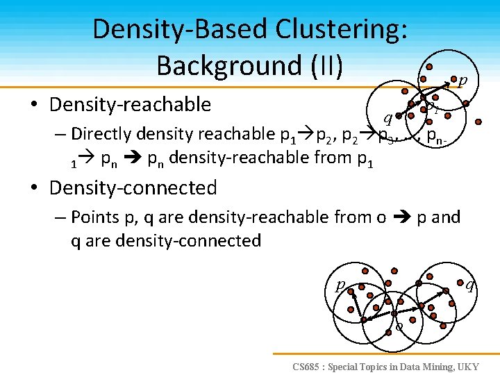
Density-Based Clustering: Background (II) • Density-reachable p p 1 q – Directly density reachable p 1 p 2, p 2 p 3, …, pn 1 pn density-reachable from p 1 • Density-connected – Points p, q are density-reachable from o p and q are density-connected p q o CS 685 : Special Topics in Data Mining, UKY

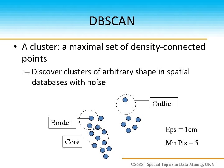
DBSCAN • A cluster: a maximal set of density-connected points – Discover clusters of arbitrary shape in spatial databases with noise Outlier Border Core Eps = 1 cm Min. Pts = 5 CS 685 : Special Topics in Data Mining, UKY

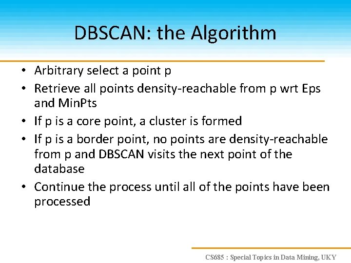
DBSCAN: the Algorithm • Arbitrary select a point p • Retrieve all points density-reachable from p wrt Eps and Min. Pts • If p is a core point, a cluster is formed • If p is a border point, no points are density-reachable from p and DBSCAN visits the next point of the database • Continue the process until all of the points have been processed CS 685 : Special Topics in Data Mining, UKY

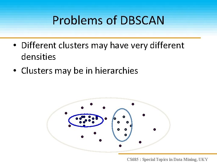
Problems of DBSCAN • Different clusters may have very different densities • Clusters may be in hierarchies CS 685 : Special Topics in Data Mining, UKY