Community Detection in Graphs Srinivasan Parthasarathy Graphs from

Community Detection in Graphs Srinivasan Parthasarathy

Graphs from the Real World Königsberg's Bridges Ref: http: //en. wikipedia. org/wiki/Seven_Bridges_of_K%C 3%B 6 nigsberg

Graphs from the Real World Zachary’s Karate Club Lusseau’s network of bottlenose dolphins

Graphs from the Real Word Webpage Hyperlink Graph Directed Communities Network of Word Associations Overlapping Communities

Real Networks Are Not Random q Degree distribution is broad, and often has a tail following power-law distribution Ref: “Plot of power-law degree distribution on log-log scale. ” From Math Insight. http: //mathinsight. org/image/power_law_degree_distribution_scatter

Real Networks Are Not Random q Edge distribution is locally inhomogeneous Community Structure!

Applications of Community Detection q q q Website mirror server assignment Recommendation system Social network role detection Functional module in biological networks Graph coarsening and summarization Network hierarchy inference

General Challenges q

Defining Motifs (Micro communities) q Local definitions: focus on the subgraph only q Clique: Vertices are all adjacent to each other q Strict definition, NP-complete problem q n-clique, n-clan, n-club, k-plex q k-core: Maximal subgraph that each vertex is adjacent to at least k other vertices in the subgraph q More advanced motifs – graphlets, k-truss etc.

Evaluating Community Quality q

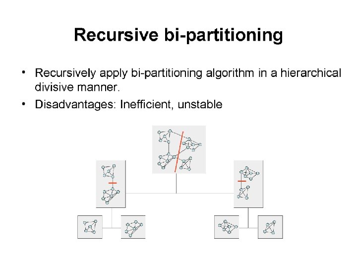
Traditional Methods q Graph Partitioning q Dividing vertices into groups of predefined size q Kernighan-Lin algorithm q Create initial bisection q Iteratively swap subsets containing equal number of vertices q Select the partition that maximize (number of edges insider modules – cut size)

Traditional Methods (Sec. 4) q Graph Partitioning q METIS (Karypis and Kumar) q Multi-level approach q Coarsen the graph into skeleton q Perform K-L and other heuristics on the skeleton q Project back with local refinement

Metis 13 q Multilevel q Use short range and G 1 long range structure nt eme refin g … … q initial partitioning q refinement … … nin q coarsening rse 3 major phases coa q Gn initial partitioning

Coarsening 14 q Find matching q related problems: q maximum (weighted) matching (O(V 1/2 E)) q minimum maximal matching (NP-hard), i. e. , matching with smallest #edges q polynomial 2 -approximations

HEM: Example

Coarsening 16 q Edge contract a b c * c

Initial Partitioning 17 q Breadth-first traversal q select k random nodes b a

Initial Partitioning 18 q Kernighan-Lin q improve partitioning by greedy swaps c d Dc = Ec – Ic = 3 – 0 = 3 Dd = Ed – Id = 3 – 0 = 3 Benefit(swap(c, d)) = Dc + Dd – 2 Acd = 3 + 3 – 2 = 4 c d

Refinement 19 q Random K-way refinement a q Randomly pick boundary node q Find new partition which reduces graph cut and maintains balance q Repeat until all boundary nodes have been visited a

Hierarchical Clustering q Graphs may have hierarchical structure q Embed vertices in a metric space and then cluster

Hierarchical Clustering q Find clusters using a similarity matrix q Agglomerative: clusters are iteratively merged if their similarity is sufficiently high q Divisive: clusters are iteratively split by removing edges with low similarity q Define similarity between clusters q Single linkage (minimum element) q Complete linkage (maximum element) q Average linkage q Drawback: dependent on similarity threshold

Other Methods q Partitional Clustering q Embed vertices in a metric space, and find clustering that optimizes the cost function q Minimum k-clustering q k-clustering sum q k-center q k-median q k-means q Fuzzy k-means q DBSCAN

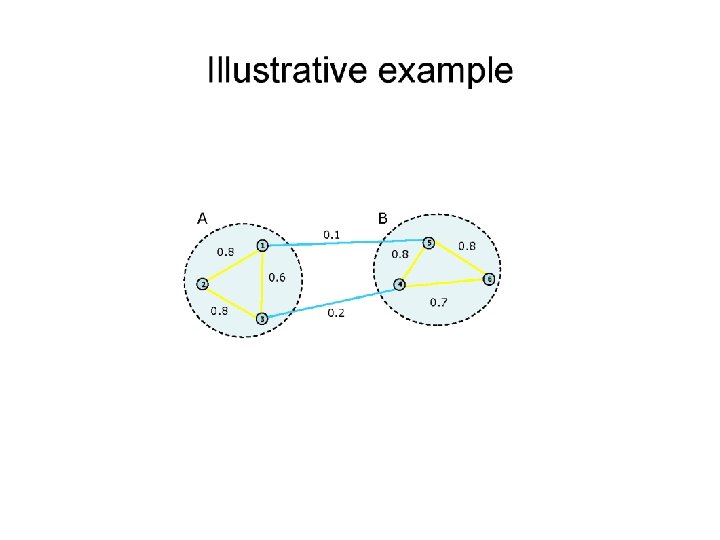
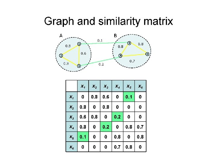
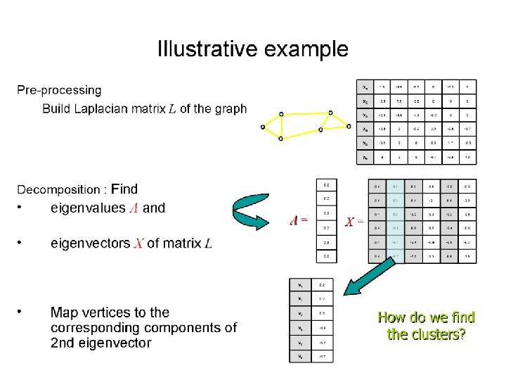
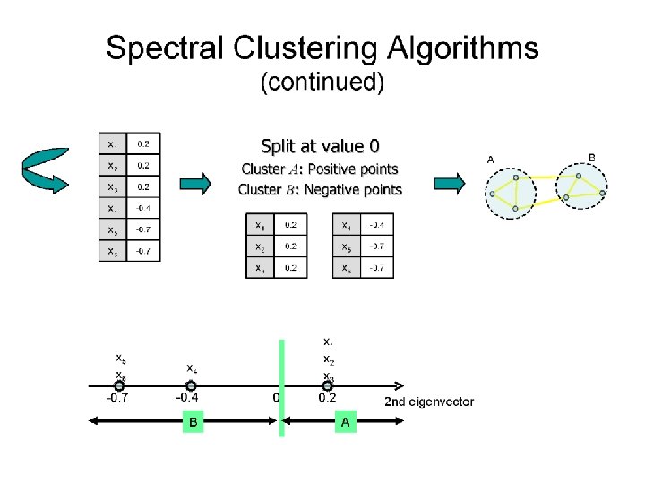
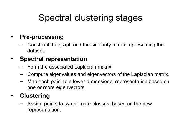
SPECTRAL CLUSTERING q

Spectral Clustering q

Alternative Approach q q Compute Laplacian as before Compute representation of each point to low rank representation by selecting several eigenvectors up to the desired inertia q Inertia Total variance explained by low rank approximation q Run k-means or any clustering algorithm on representation

Variants of Betweenness q q Girvan and Newman’s edge centrality algorithm: Iteratively remove edges with high centrality and re-compute the values Define edge centrality: Edge betweenness: number of all-pair shortest paths that run along an edge q Random-walk betweenness: probability of random walker passing the edge q Current-flow betweenness: current passing the edge in a unit resistance network q q

Random Walk Based Approaches q q q A random walker spends a long time inside a community due to the high density of internal edges E. g. 1 : Zhou used random walks to dene a distance between pairs of vertices the distance between i and j is the average number of edges that a random walker has to cross to reach j starting from i.

Stochastic (Flow) Matrix: A matrix where each column sums to 1. Stochastic Flow: An entry in a stochastic matrix, interpreted as the “flow” or “transition probability”. 1 1 2 4 4 34 3 0. 33 0. 5 3 3 2 0. 5 1. 0 0. 33 4 0. 5

Stochastic (Flow) Matrix: A matrix where each column sums to 1. Stochastic Flow: An entry in a stochastic matrix, interpreted as the “flow” or “transition probability”. 1 1 2 4 4 0. 5 0. 33 4 0. 5 1. 0 Flow from 2 to 3 37 3 0. 33 3 3 2 0. 5

Stochastic (Flow) Matrix: A matrix where each column sums to 1. Stochastic Flow: An entry in a stochastic matrix, interpreted as the “flow” or “transition probability”. 1 1 2 1 0. 33 0. 25 2 0. 33 0. 25 0. 5 2 3 3 In-flows of 2 4 0. 33 0. 25 3 4 0. 33 4 Out-flows of 2 39

Repeatedly apply certain operations to the flow matrix until the matrix converges and can be interpreted as a clustering. 1 2 1. 0 3 4 1 2 3 3 4 4 40 1. 0

Markov Clustering (MCL) Stijn van Dongen, 2000 The original Stochastic flow clustering algorithm 41

The MCL algorithm Create initial flow matrix M from input Expand flow out to new, well-connected nodes. Expand M : = M * M Raise each entry to the power r. Increase inequality in each column. Inflate M : = M. ^r (r > 1) Remove entries in matrix close to zero. Prune No Converged? Yes Output Clusters 42

[van Dongen ’ 00] 43

MCL Flaws 1. Outputs many small clusters. 2. Does not scale well. [Chakrabarti and Faloutsos ‘ 06] 44

MCL Flaws 1. Outputs many small clusters. Fix: Regularized MCL 2. Does not scale well. Fix: Multi-Level Regularized MCL 45

The Regularize operator Key idea: Set the out-flows of a node so as to minimize “distance” from neighbors. Distance measured using KL-divergence. Closed-form solution! Weight of neighbor j In matrix notation, 47

The R-MCL algorithm Create initial flow matrix M from input Take into account out-flows of neighbors. Regularize M : = W * M Raise each entry to the power r. Increase inequality in each column. Inflate M : = M. ^r (r > 1) Remove entries in matrix close to zero. Prune No Converged? Yes Output Clusters 49

MCL R-MCL [Automtically visualized using Prefuse] 50

Multi-Level Regularized MCL Making R-MCL fast 51

General idea of multi-level methods: Create smaller “replicas” of the original problem. Solving the smaller problem should help us solve the original problem. [Shang-hua Teng ’ 97] 52

“Coarsening”: Creating smaller replicas Input Graph Coarsened Graph 1 3 2 4 1 2 2 [Karypis and Kumar ’ 98] 53 5 1 3

Output clusters Input Graph Coarsen Input Graph Run R-MCL, Uncoarsen, Initalize bigger flow matrix . . . Captures global graph topology! Coarsest Graph 54 Faster to run on smaller graphs first!

Comparison with MCL on Protein Interaction Networks Dataset (n, m) Quality Change Speedup (Time) Yeast (5 k, 15 k) 36% 2. 5 x (0. 4 s) Yeast_Noisy (6 k, 200 k) 300% 57 x (8 s) Human (10 k, 60 k) 21. 6% 200 x (2 s) [Hardware: Quad-core Intel i 5 CPU, 3. 2 GHz, with 16 GB RAM ] 55

Wikipedia article-article network ~1. 1 M nodes, ~53 M edges Quality (Absolute) Time (minutes) MLR-MCL 20. 2 132 Metis 12. 3 125 Metis+MQI 19. 2 592 Note: MCL and other methods timed-out or ran out of memory. [Hardware: Quad-core Intel i 5 CPU, 3. 2 GHz, with 16 GB RAM ] 58

Real World Impact “ . . . . ” 59

Overlapping community detection q Most of previous methods can only generate nonoverlapped clusters. q A node only belongs to one community. q Not real in many scenarios. q q A person usually belongs to multiple communities. Most of current overlapping community detection algorithms can be categorized into three groups. q Mainly based on non-overlapping communities algorithms. 60

Overlapping community detection q 1. Identifying bridge nodes q First, identifying bridge nodes and remove or duplicate these nodes. q q Duplicate nodes have connection b/t them. Then, apply hard clustering algorithm. q If bridge nodes was removed, add them back. E. g. DECAFF [Li 2007], Peacock [Gregory 2009] q Cons: Only a small part of nodes can be identified as bridge nodes. q 2 1 5 4 3 6 61

Overlapping community detection q 2. Line graph transformation q Edges become nodes. q New nodes have connection if they originally share a node. q Then, apply hard clustering algorithm on the line graph. q E. g. Link. Community [Ahn 2010] q Cons: An edge can only belong to one cluster 1 1 2 2 4 4 3 3 6 5 5 8 7 6 62

Overlapping community detection q 3. Local clustering q (optional) Select seed nodes. q Expand seed node according to some criterion. q E. g. Cluster. One [Nepusz 2012], MCODE [Bader 2003], CPM [Adamcsek 2006], RRW [Macropol 2009] q Cons: Not globally consider the topology 2 1 5 4 3 6 63

Dynamic community q Cluster each snapshot independently q Then mapping clusters in each clustering. q q If two clusters in continuous snapshots share most of nodes, then the next one evolves from the previous one. Detect the evolution of communities in a dynamic graph. q Birth, Death, Growth, Contraction, Merge, Split. 64

Dynamic community 65

Dynamic community q q Asur et al. (2007) further detect a event involving nodes. q E. g. join and leave q Measure the node behavior. q Sociability: How frequently a node join and leave a community. q Influence: How a node can influence other nodes’ activities. Usage q Understand the community behavior. q E. g. age is positively correlated with the size. q Predict the evolution of a community q Predict node (user) behavior, predict link 66

Dynamic community detection q Hypothesis: Communities in dynamic graphs are “smooth”. q q Detect communities by also considering the previous snapshots. Chakrabarti et al (2006) introduce history cost. q Measures the dissimilarity between two clusterings in continuous timestamps. q A smooth clustering has lower history cost. q Add this cost to the objective function. 67

COMMUNITY DISCOVERY IN DIRECTED GRAPHS • Research on graph clustering is mostly focused on undirected graphs, yet the graphs from a number of domains are directed in nature. Web graphs Citation networks Twitter (follower) network • Undirected edges indicate similarity/affinity while directed edges need not indicate similarity. It is important to recognize this difference when clustering. Venu Satuluri and Srinivasan Parthasarathy |Symmetrizations for Clustering Directed Graphs

Existing research Objective functions such as normalized cuts, originally meant for undirected graphs, have been extended to directed graphs [Zhou et al. ’ 05, Huang et al. ‘ 06, Meila ‘ 07] The Ncut (normalized cut) of a cluster S is the probability of a random walk escaping from S to the rest of the graph , or vice versa. Clusters with low Ncut are found by spectral methods i. e. by post-processing the eigenvectors of the directed Laplacian of the graph. Venu Satuluri and Srinivasan Parthasarathy |Symmetrizations for Clustering Directed Graphs

Drawbacks of Existing Research Existing measures are biased to find groups of nodes with high inter-connectivity. However, directed networks often contain clusters which need not be well inter-connected in the original graph! Example: Nodes 4 and 5 form a cluster, even though they are not connected to one another. Real-life analogue: Research papers written on the same topic in a short span of time may not be able to cite one another but may cite (and be cited by) a common set of papers. Venu Satuluri and Srinivasan Parthasarathy |Symmetrizations for Clustering Directed Graphs

Our Framework Directed Graph Symmetrizations Existing • A+AT • Random walk Proposed • Bibliometric • Degree -discounted (Weighted) Undirected Graph Clustering Algorithms • MLR-MCL • Metis • Graclus • Spectral Clusters By “Symmetrizations”, we mean procedures for transforming a directed graph into an undirected graph. Venu Satuluri and Srinivasan Parthasarathy |Symmetrizations for Clustering Directed Graphs

Why a two-stage framework? Why convert to an undirected graph, and then cluster the undirected graph? Three reasons: 1. Our framework makes the underlying similarity assumptions explicit. 2. Flexibility: prior methods which directly cluster directed graphs can be re-expressed in our framework. 3. Decouples similarity measure and clustering algorithm, thereby allows use of latest and most suitable clustering algorithms. Venu Satuluri and Srinivasan Parthasarathy |Symmetrizations for Clustering Directed Graphs

Existing symmetrizations Let the adjacency matrix of the input directed graph be A. • A+AT symmetrization : • Corresponds to ignoring directionality. • Implicit symmetrization that is used widely. • Random Walk symmetrization: • The directed graph G can be converted into an undirected graph GU so that the normalized cut on GU is equal to the normalized cut on G. [Gleich ‘ 06] • P is the Markov transition matrix, and Π is a diagonal matrix with the stationary distribution (Page. Rank) on the diagonal. • Clustering GU is equivalent to the algorithms proposed by [Zhou ‘ 05, Huang ’ 06] Venu Satuluri and Srinivasan Parthasarathy |Symmetrizations for Clustering Directed Graphs

Proposed symmetrizations - Bibliometric Our Approach: Design a suitable similarity measure for pairs of vertices, and set the edge weight between a pair of vertices in the symmetrized graph to be their similarity. Axioms for similarity: Axiom 1: Vertices are similar if they point to or are pointed at by common vertices. Similarity(i, j) = No. of shared in-links + No. of shared out-links Symmetrized graph GU = ATA + AAT We call this Bibliometric symmetrization (for historic reasons) Venu Satuluri and Srinivasan Parthasarathy |Symmetrizations for Clustering Directed Graphs

Proposed Symmetrizations - Degree-discounted Disadvantage of Bibliometric: Hub nodes can have spuriously high similarity with a lot of nodes. We propose Degree-discounted similarity incorporating the below axioms also: Axiom 2: Commonly pointing to nodes with high in-degree counts for less than pointing to nodes with low in-degree. Axiom 3: Being pointed at by nodes with high out-degree counts for less than being pointed at by nodes with low out-degree. Venu Satuluri and Srinivasan Parthasarathy |Symmetrizations for Clustering Directed Graphs

Proposed Symmetrizations - Degree-discounted A – Adjacency matrix of input directed graph Do – Diagonal matrix with out-degrees, Di – Diagonal matrix with in-degrees Degree-discounted out-link similarity Od between i and j: α and β are the degree-discounting exponents. Similarly, degree-discounted in-link similarity Id can be derived as: Final degree-discounted similarity matrix: We found α=β=0. 5 to work best empirically (similar to L 2 -normalization). Venu Satuluri and Srinivasan Parthasarathy |Symmetrizations for Clustering Directed Graphs

Pruning Thresholds For Bibliometric & Degree-discounted, it is critical to prune the symmetrized matrix i. e. remove edges below a threshold. Two reasons: 1. The full symmetrized matrix is very dense and is difficult to both compute, as well as cluster subsequently. 2. The symmetrization itself can be computed much faster if we only want entries above a certain threshold • Large literature on speeding up all-pairs similarity computation in the presence of a threshold e. g. [Bayardo et. al. , WWW ‘ 07] It is much easier to set pruning thresholds for Degree-discounted compared to Bibliometric. Venu Satuluri and Srinivasan Parthasarathy |Symmetrizations for Clustering Directed Graphs

Experiments Datasets: 1. Cora: Citation network of ~17, 000 CS research papers. Classified manually into 70 research areas. (Thanks to Andrew Mc. Callum. ) 2. Wikipedia: Article-article hyperlink graph with 1. 1 Million nodes. Category assignments at bottom of each article used as the ground truth. Evaluation Metric: Avg. F score = Weighted Average of F scores of individual clusters. F score of a cluster = Harmonic mean of Precision and Recall w. r. t. ground truth cluster (the best matched one). Algorithms for clustering symmetrized graphs: MLR-MCL [Satuluri and Parthasarathy ’ 09] Graclus [Dhillon et al. ’ 07] Metis [Karypis and Kumar ’ 98] Venu Satuluri and Srinivasan Parthasarathy |Symmetrizations for Clustering Directed Graphs

Results on Cora – Comparison with Best. WCut Degree-discounted is 2 -3 orders of magnitude faster and also gives higher-quality clusters compared to Best. WCut [Meila & Pentney ‘ 07]. Venu Satuluri and Srinivasan Parthasarathy |Symmetrizations for Clustering Directed Graphs

Results on Cora – Comparison of Symmetrizations Degree-discounted performs the best among all symmetrizations, when used with either MLR-MCL or Graclus. Venu Satuluri and Srinivasan Parthasarathy |Symmetrizations for Clustering Directed Graphs

Results on Wikipedia (Quality) MLR-MCL and Metis show improvements of 12% and 25% on the Degreediscounted graph over the baseline. Venu Satuluri and Srinivasan Parthasarathy |Symmetrizations for Clustering Directed Graphs

Timing results on Wikipedia Both MLR-MCL and Metis run 2 -4 times faster on Degree-discounted similarity graph. Venu Satuluri and Srinivasan Parthasarathy |Symmetrizations for Clustering Directed Graphs

Degree distribution on Wikipedia Venu Satuluri and Srinivasan Parthasarathy |Symmetrizations for Clustering Directed Graphs

Example Wikipedia cluster Venu Satuluri and Srinivasan Parthasarathy |Symmetrizations for Clustering Directed Graphs

Top similarity pairs in Wikipedia Venu Satuluri and Srinivasan Parthasarathy |Symmetrizations for Clustering Directed Graphs

Testing algorithms q 1. Real data w/o gold standards: q 2. Read data w/ gold standard q 3. Synthetic data q Hard to say which algorithm is the best. q q In different scenarios, different algorithms might be best choices. 1 and 2 are practical, but hard to determine which kinds of graphs / clusters an algorithm is suitable. q Sparse/Dense, power-law, overlapping communities. 86

Real data w/o gold standards q q q Almeida et al. (2011) discuss many metrics. Modularity, normalized cut, Silhouette Index, conductance, etc. Each metric has its own bias. q q Modularity, conductance are biased toward small number of clusters. Should not choose the algorithms which is designed for that metric, e. g. modularity-based method. 87

Real data w/ gold standard q q Examples of gold standard clusters q “Network”tags in Facebook. q Article tags in Wiki q Protein annotations. Evaluate how closely the clusters are matched to the gold standard. Cons: Overfitting – biased towards the clustering with similar cluster size. Cons: Gold standard might be noisy, incomplete. 88

Metrics q q F-measure q Harmonic mean of precision and recall q Need a parameter θ (usually 0. 25) Accuracy q Square root of PPV * Sn q Tij: common nodes in community I and cluster j 89

Metrics q q Normalized Mutual Information q H(X): Entropy of X q I(X, Y): H(X) – H(X|Y), H(X|Y) is the conditional entropy Some metrics need to be adjusted for overlapping clustering. 90

Synthetic data q Girvan and Newman (2002) Benchmark q Fixed 128 nodes and 4 communities q Can tune noisy level q Cons: All nodes have the same expected degree; All communities have the same size, etc 91

Synthetic data q LFR (Lancichinetti 2009) q Generate power-law, weighted/unweighted, directed/undirected graph with gold standard q Pros: can generate variaous graphs. q q q # nodes, average degree, power-law exponent. q Average/Min/Max community size, # bridge nodes. q Noisy level, etc. Cons: The number of communities each bridge nodes belonging to is fixed. Use the above metrics to evaluate the result. 92