Face detection Face detection Stateoftheart face detection demo

Face detection

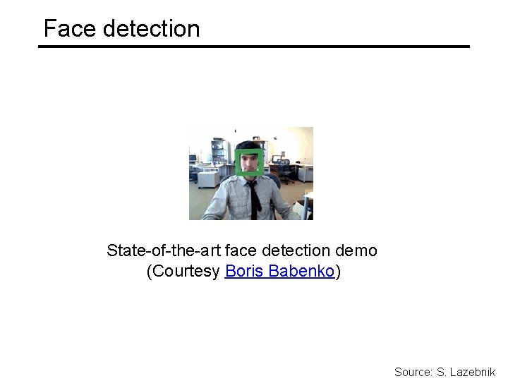
Face detection State-of-the-art face detection demo (Courtesy Boris Babenko) Source: S. Lazebnik

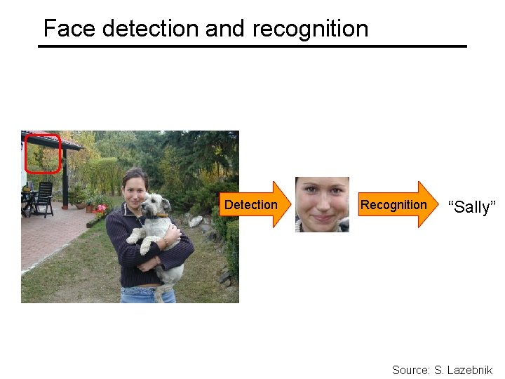
Face detection and recognition Detection Recognition “Sally” Source: S. Lazebnik

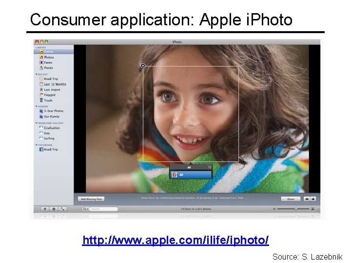
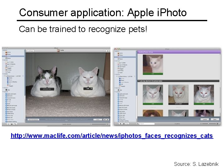
Consumer application: Apple i. Photo http: //www. apple. com/ilife/iphoto/ Source: S. Lazebnik

Consumer application: Apple i. Photo Can be trained to recognize pets! http: //www. maclife. com/article/news/iphotos_faces_recognizes_cats Source: S. Lazebnik

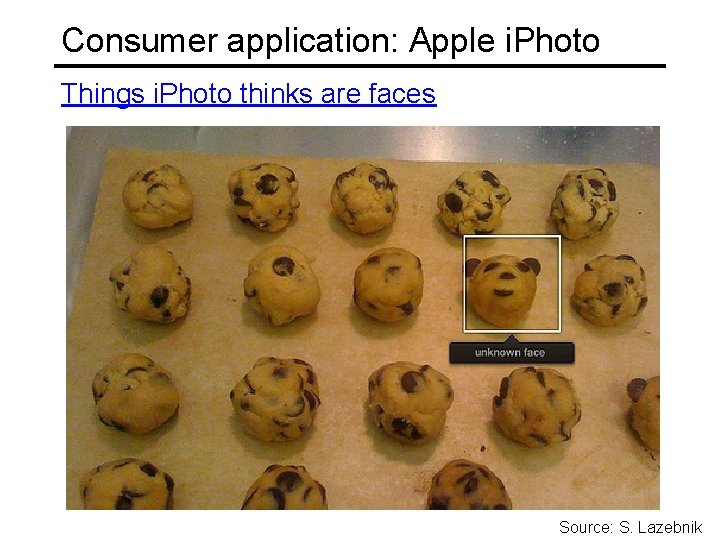
Consumer application: Apple i. Photo Things i. Photo thinks are faces Source: S. Lazebnik

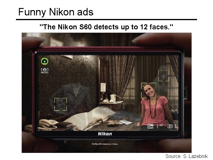
Funny Nikon ads "The Nikon S 60 detects up to 12 faces. " Source: S. Lazebnik

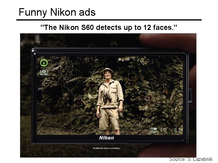
Funny Nikon ads "The Nikon S 60 detects up to 12 faces. " Source: S. Lazebnik

Challenges of face detection • Sliding window detector must evaluate tens of thousands of location/scale combinations • Faces are rare: 0– 10 per image • A megapixel image has ~106 pixels and a comparable number of candidate face locations • For computational efficiency, we should try to spend as little time as possible on the non-face windows • To avoid having a false positive in every image, our false positive rate has to be less than 10 -6 Source: S. Lazebnik

The Viola/Jones Face Detector • A seminal approach to real-time object detection • Training is slow, but detection is very fast • Key ideas • Integral images for fast feature evaluation • Boosting for feature selection • Attentional cascade for fast rejection of non-face windows P. Viola and M. Jones. Rapid object detection using a boosted cascade of simple features. CVPR 2001. P. Viola and M. Jones. Robust real-time face detection. IJCV 57(2), 2004. Source: S. Lazebnik

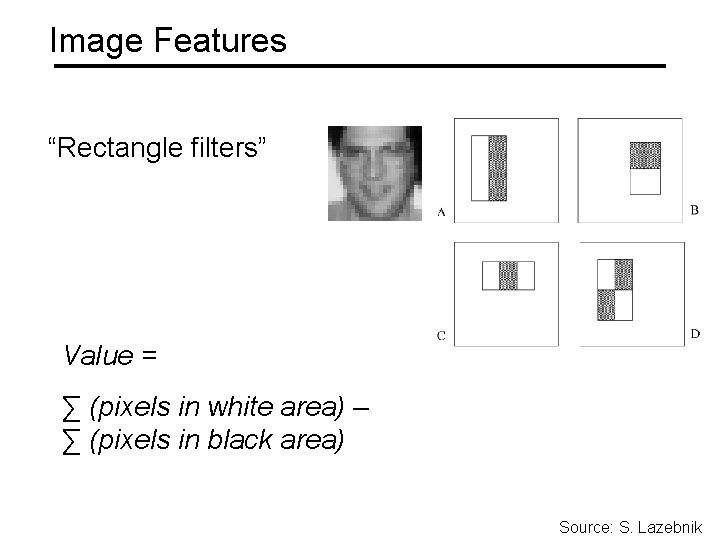
Image Features “Rectangle filters” Value = ∑ (pixels in white area) – ∑ (pixels in black area) Source: S. Lazebnik

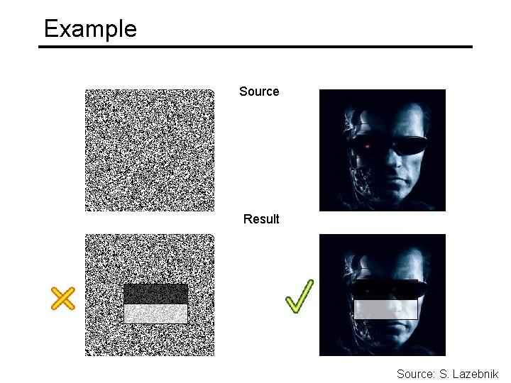
Example Source Result Source: S. Lazebnik

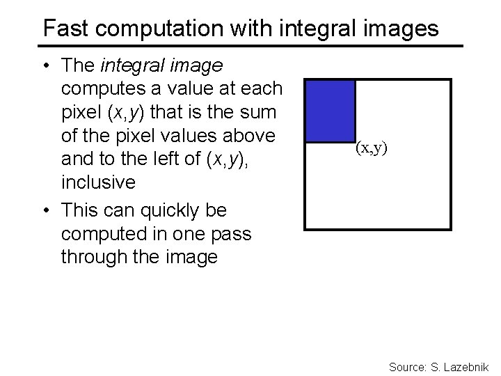
Fast computation with integral images • The integral image computes a value at each pixel (x, y) that is the sum of the pixel values above and to the left of (x, y), inclusive • This can quickly be computed in one pass through the image (x, y) Source: S. Lazebnik

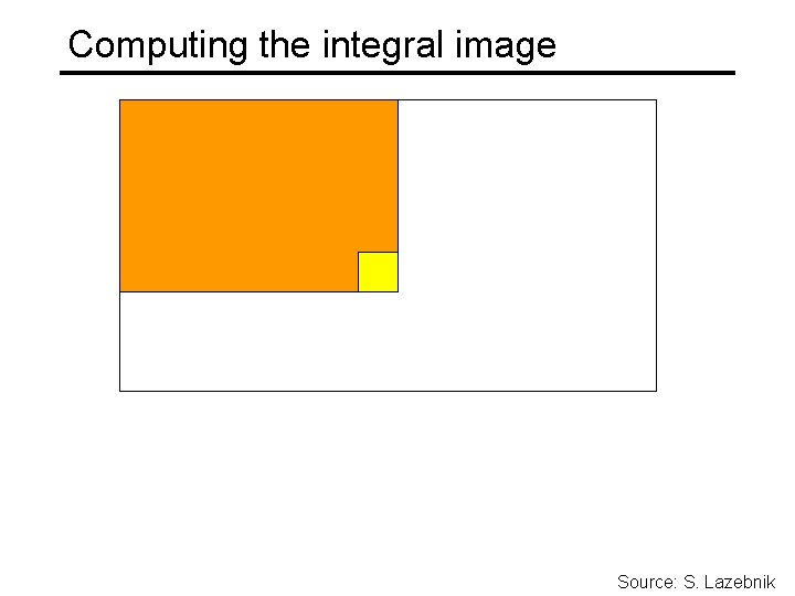
Computing the integral image Source: S. Lazebnik

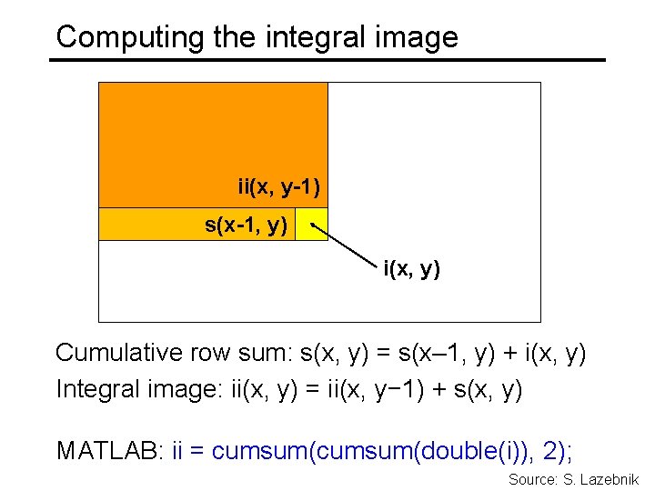
Computing the integral image ii(x, y-1) s(x-1, y) i(x, y) Cumulative row sum: s(x, y) = s(x– 1, y) + i(x, y) Integral image: ii(x, y) = ii(x, y− 1) + s(x, y) MATLAB: ii = cumsum(double(i)), 2); Source: S. Lazebnik

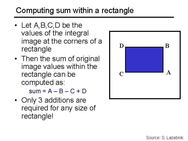
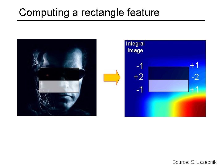
Computing sum within a rectangle • Let A, B, C, D be the values of the integral image at the corners of a rectangle • Then the sum of original image values within the rectangle can be computed as: D B C A sum = A – B – C + D • Only 3 additions are required for any size of rectangle! Source: S. Lazebnik

Computing a rectangle feature Integral Image -1 +2 -1 +1 -2 +1 Source: S. Lazebnik

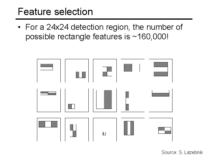
Feature selection • For a 24 x 24 detection region, the number of possible rectangle features is ~160, 000! Source: S. Lazebnik

Feature selection • For a 24 x 24 detection region, the number of possible rectangle features is ~160, 000! • At test time, it is impractical to evaluate the entire feature set • Can we create a good classifier using just a small subset of all possible features? • How to select such a subset? Source: S. Lazebnik

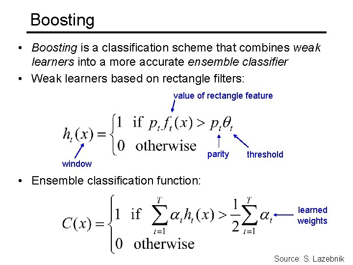
Boosting • Boosting is a classification scheme that combines weak learners into a more accurate ensemble classifier • Weak learners based on rectangle filters: value of rectangle feature window parity threshold • Ensemble classification function: learned weights Source: S. Lazebnik

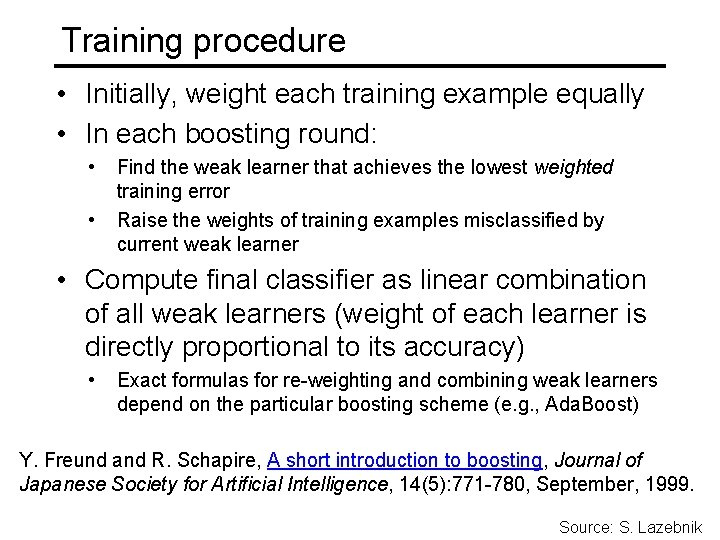
Training procedure • Initially, weight each training example equally • In each boosting round: • • Find the weak learner that achieves the lowest weighted training error Raise the weights of training examples misclassified by current weak learner • Compute final classifier as linear combination of all weak learners (weight of each learner is directly proportional to its accuracy) • Exact formulas for re-weighting and combining weak learners depend on the particular boosting scheme (e. g. , Ada. Boost) Y. Freund and R. Schapire, A short introduction to boosting, Journal of Japanese Society for Artificial Intelligence, 14(5): 771 -780, September, 1999. Source: S. Lazebnik

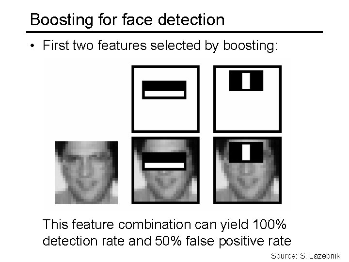
Boosting for face detection • First two features selected by boosting: This feature combination can yield 100% detection rate and 50% false positive rate Source: S. Lazebnik

Boosting • Advantages of boosting • Flexibility in the choice of weak learners, boosting scheme • Testing is fast • Easy to implement • Disadvantages • Needs many training examples • Training is slow Source: S. Lazebnik

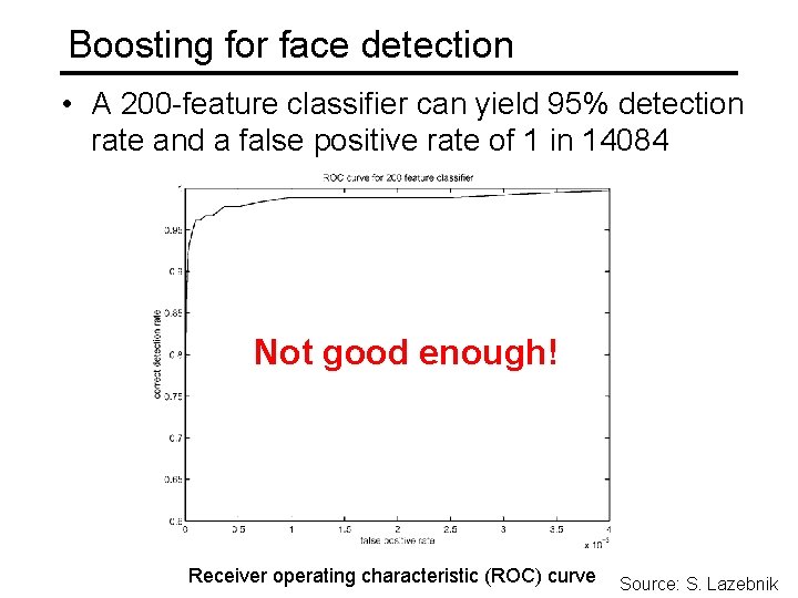
Boosting for face detection • A 200 -feature classifier can yield 95% detection rate and a false positive rate of 1 in 14084 Not good enough! Receiver operating characteristic (ROC) curve Source: S. Lazebnik

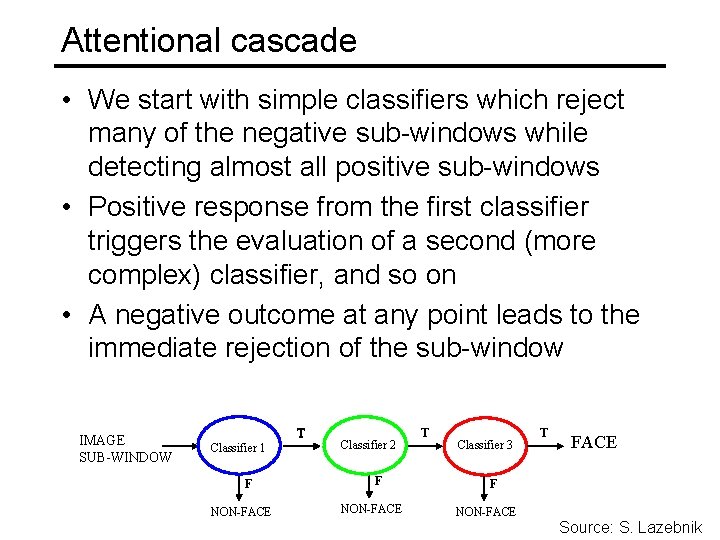
Attentional cascade • We start with simple classifiers which reject many of the negative sub-windows while detecting almost all positive sub-windows • Positive response from the first classifier triggers the evaluation of a second (more complex) classifier, and so on • A negative outcome at any point leads to the immediate rejection of the sub-window IMAGE SUB-WINDOW T Classifier 1 F NON-FACE Classifier 2 F NON-FACE T Classifier 3 T FACE F NON-FACE Source: S. Lazebnik

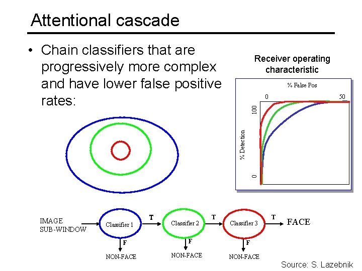
Attentional cascade • Chain classifiers that are progressively more complex and have lower false positive rates: Receiver operating characteristic % False Pos 0 50 0 % Detection 100 vs false neg determined by IMAGE SUB-WINDOW T Classifier 1 F NON-FACE Classifier 2 F NON-FACE T Classifier 3 T FACE F NON-FACE Source: S. Lazebnik

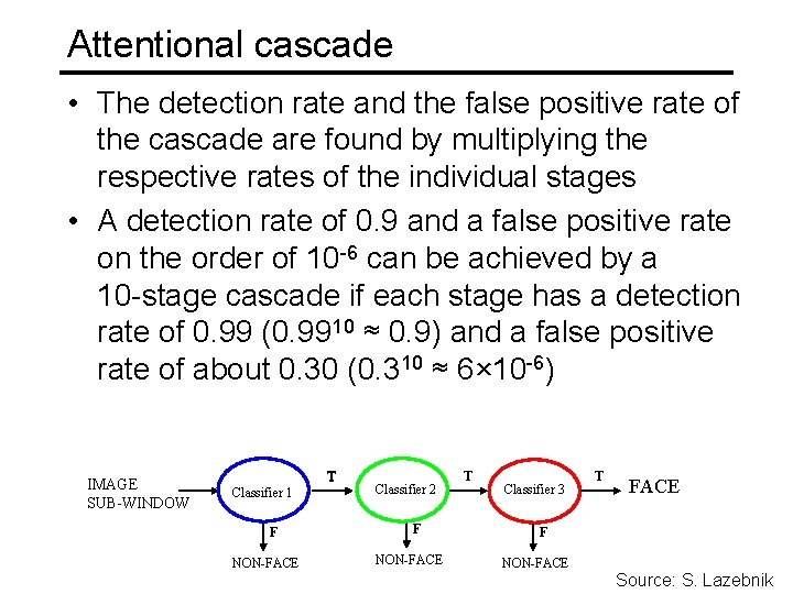
Attentional cascade • The detection rate and the false positive rate of the cascade are found by multiplying the respective rates of the individual stages • A detection rate of 0. 9 and a false positive rate on the order of 10 -6 can be achieved by a 10 -stage cascade if each stage has a detection rate of 0. 99 (0. 9910 ≈ 0. 9) and a false positive rate of about 0. 30 (0. 310 ≈ 6× 10 -6) IMAGE SUB-WINDOW T Classifier 1 F NON-FACE Classifier 2 F NON-FACE T Classifier 3 T FACE F NON-FACE Source: S. Lazebnik

Training the cascade • Set target detection and false positive rates for each stage • Keep adding features to the current stage until its target rates have been met • Need to lower Ada. Boost threshold to maximize detection (as opposed to minimizing total classification error) • Test on a validation set • If the overall false positive rate is not low enough, then add another stage • Use false positives from current stage as the negative training examples for the next stage Source: S. Lazebnik

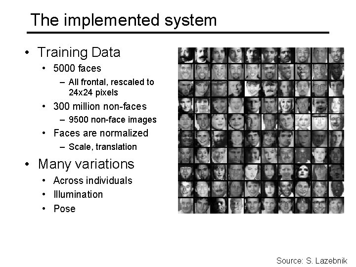
The implemented system • Training Data • 5000 faces – All frontal, rescaled to 24 x 24 pixels • 300 million non-faces – 9500 non-face images • Faces are normalized – Scale, translation • Many variations • Across individuals • Illumination • Pose Source: S. Lazebnik

System performance • Training time: “weeks” on 466 MHz Sun workstation • 38 layers, total of 6061 features • Average of 10 features evaluated per window on test set • “On a 700 Mhz Pentium III processor, the face detector can process a 384 by 288 pixel image in about. 067 seconds” • 15 Hz • 15 times faster than previous detector of comparable accuracy (Rowley et al. , 1998) Source: S. Lazebnik

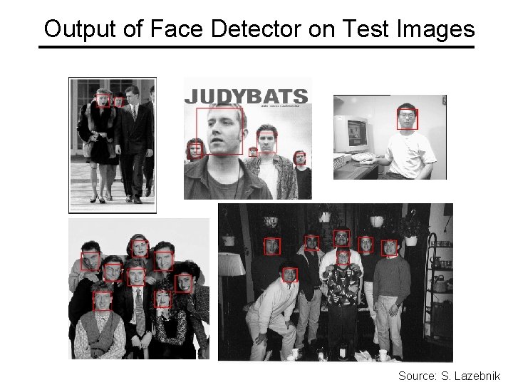
Output of Face Detector on Test Images Source: S. Lazebnik

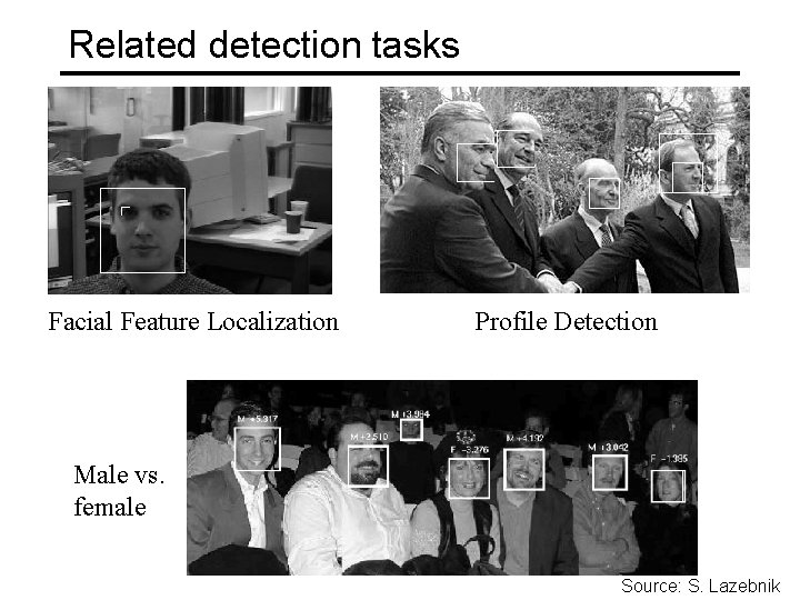
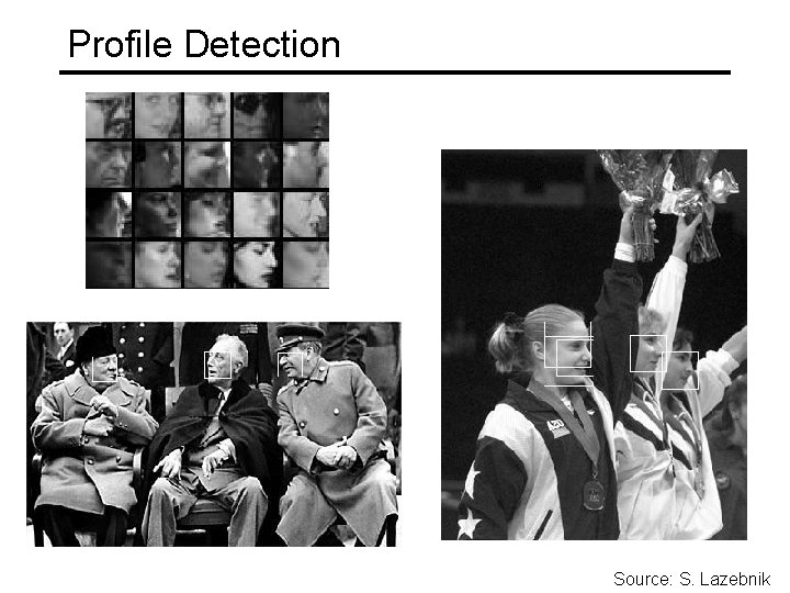
Related detection tasks Facial Feature Localization Profile Detection Male vs. female Source: S. Lazebnik

Profile Detection Source: S. Lazebnik

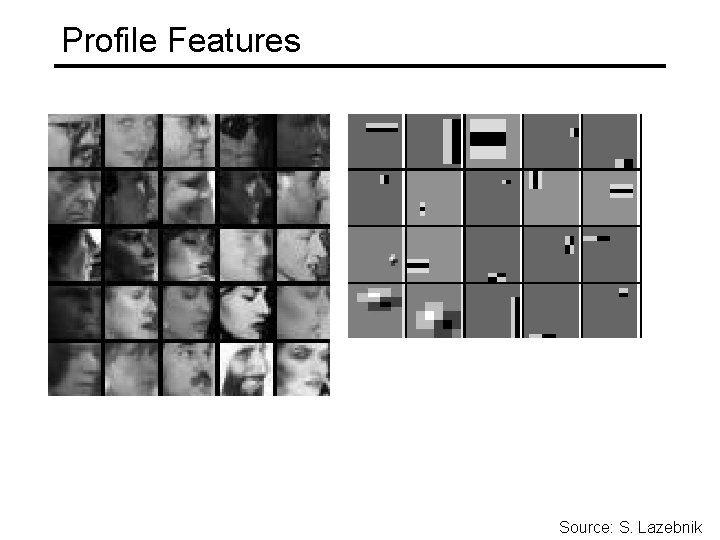
Profile Features Source: S. Lazebnik

Summary: Viola/Jones detector • • Rectangle features Integral images for fast computation Boosting for feature selection Attentional cascade for fast rejection of negative windows Source: S. Lazebnik

Face detection and recognition Detection Recognition “Sally” Source: S. Lazebnik

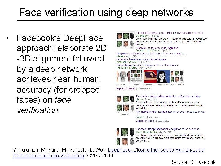
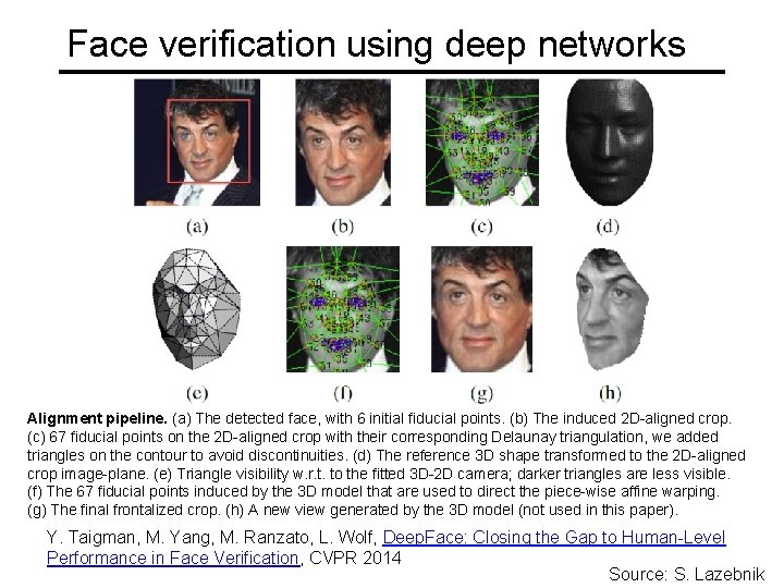
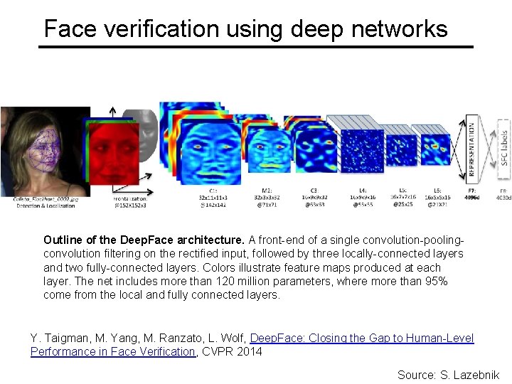
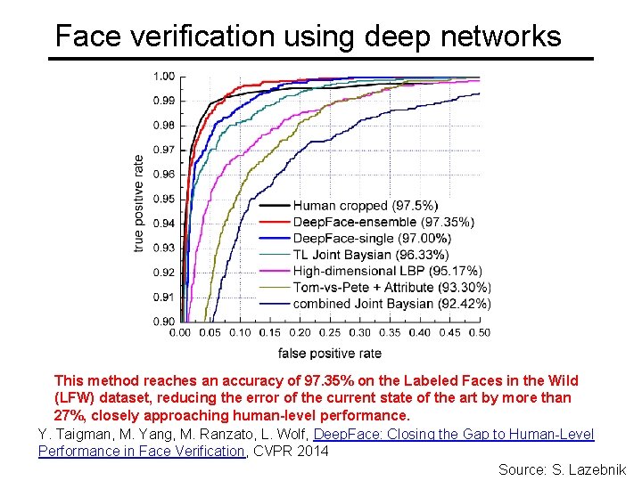
Face verification using deep networks • Facebook’s Deep. Face approach: elaborate 2 D -3 D alignment followed by a deep network achieves near-human accuracy (for cropped faces) on face verification Y. Taigman, M. Yang, M. Ranzato, L. Wolf, Deep. Face: Closing the Gap to Human-Level Performance in Face Verification, CVPR 2014 Source: S. Lazebnik

Face verification using deep networks Alignment pipeline. (a) The detected face, with 6 initial fiducial points. (b) The induced 2 D-aligned crop. (c) 67 fiducial points on the 2 D-aligned crop with their corresponding Delaunay triangulation, we added triangles on the contour to avoid discontinuities. (d) The reference 3 D shape transformed to the 2 D-aligned crop image-plane. (e) Triangle visibility w. r. t. to the fitted 3 D-2 D camera; darker triangles are less visible. (f) The 67 fiducial points induced by the 3 D model that are used to direct the piece-wise affine warping. (g) The final frontalized crop. (h) A new view generated by the 3 D model (not used in this paper). Y. Taigman, M. Yang, M. Ranzato, L. Wolf, Deep. Face: Closing the Gap to Human-Level Performance in Face Verification, CVPR 2014 Source: S. Lazebnik

Face verification using deep networks Outline of the Deep. Face architecture. A front-end of a single convolution-poolingconvolution filtering on the rectified input, followed by three locally-connected layers and two fully-connected layers. Colors illustrate feature maps produced at each layer. The net includes more than 120 million parameters, where more than 95% come from the local and fully connected layers. Y. Taigman, M. Yang, M. Ranzato, L. Wolf, Deep. Face: Closing the Gap to Human-Level Performance in Face Verification, CVPR 2014 Source: S. Lazebnik

Face verification using deep networks This method reaches an accuracy of 97. 35% on the Labeled Faces in the Wild (LFW) dataset, reducing the error of the current state of the art by more than 27%, closely approaching human-level performance. Y. Taigman, M. Yang, M. Ranzato, L. Wolf, Deep. Face: Closing the Gap to Human-Level Performance in Face Verification, CVPR 2014 Source: S. Lazebnik