Classification Numerical classifiers Introduction to Data mining PangNing

Classification Numerical classifiers Introduction to Data mining Pang-Ning Tan, Michael Steinbach, Vipin Kumar Presented by: Ding-Ying Chiu Date: 2008/10/17 0

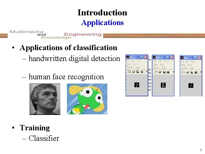
Introduction Applications • Applications of classification – handwritten digital detection – human face recognition • Training – Classifier 1

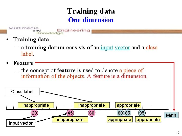
Training data One dimension • Training data – a training datum consists of an input vector and a class label. • Feature – the concept of feature is used to denote a piece of information of the objects. A feature is a dimension. Class label inappropriate 20 Input vector inappropriate 45 inappropriate 60 appropriate 80 85 appropriate 95 appropriate Math 2

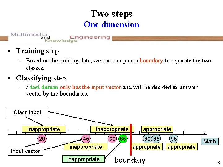
Two steps One dimension • Training step – Based on the training data, we can compute a boundary to separate the two classes. • Classifying step – a test datum only has the input vector and will be decided its answer vector by the boundaries. Class label inappropriate 20 Input vector inappropriate 45 inappropriate 60 65 appropriate 80 85 appropriate boundary 95 appropriate Math 3

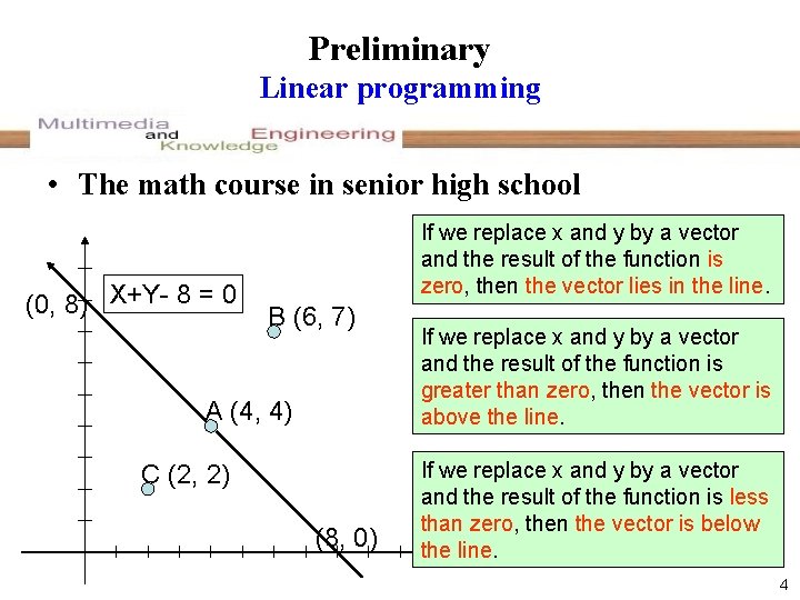
Preliminary Linear programming • The math course in senior high school (0, 8) X+Y- 8 = 0 If we replace x and y by a vector and the result of the function is zero, then the vector lies in the line. B (6, 7) A (4, 4) C (2, 2) (8, 0) If we replace x and y by a vector and the result of the function is greater than zero, then the vector is above the line. If we replace x and y by a vector and the result of the function is less than zero, then the vector is below the line. 4

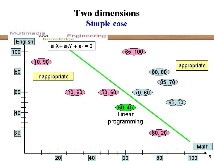
Two dimensions Simple case English a 1 X+ a 2 Y + a 3 = 0 100 65, 100 10, 90 80 appropriate 80, 80 inappropriate 60 85, 70 30, 60 50, 60 70, 60 95, 50 60, 45 40 Linear programming 80, 20 20 Math 20 40 60 80 100 5

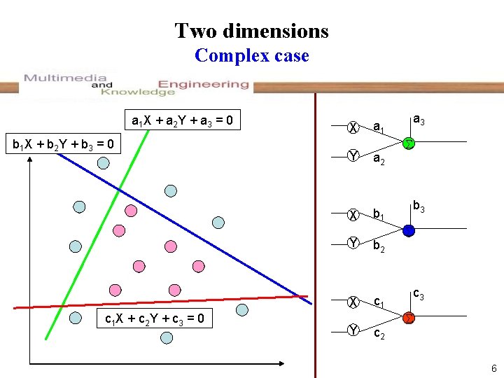
Two dimensions Complex case a 1 X + a 2 Y + a 3 = 0 b 1 X + b 2 Y + b 3 = 0 c 1 X + c 2 Y + c 3 = 0 X Y a 2 X b 1 Y b 2 X c 1 Y a 3 a 1 c 2 b 3 c 3 6

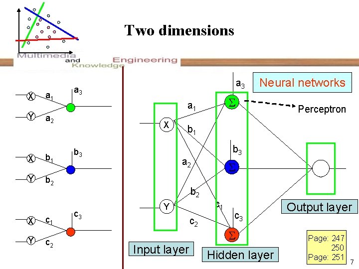
Two dimensions X Y a 1 b 1 Y b 2 X c 1 Y c 2 X b 3 Perceptron b 1 b 3 a 2 b 2 c 3 Neural networks a 1 a 2 X a 3 Y c 2 Input layer c 1 c 3 Hidden layer Output layer Page: 247 250 Page: 251 7

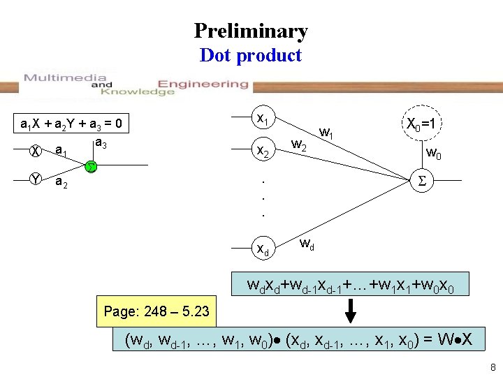
Preliminary Dot product x 1 a 1 X + a 2 Y + a 3 = 0 a 3 X a 1 Y a 2 x 2 w 2 . . . xd w 1 X 0=1 w 0 wd wdxd+wd-1 xd-1+…+w 1 x 1+w 0 x 0 Page: 248 – 5. 23 (wd, wd-1, …, w 1, w 0) (xd, xd-1, …, x 1, x 0) = W X 8

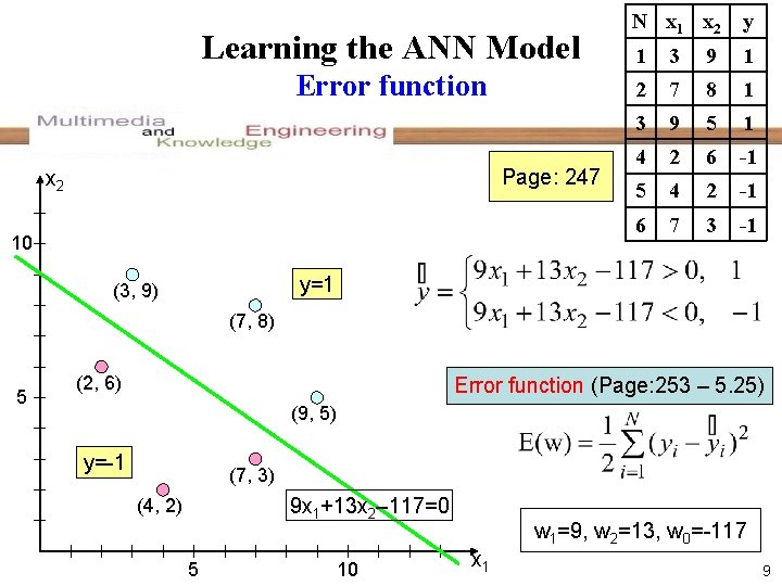
Learning the ANN Model Error function Page: 247 x 2 10 N x 1 x 2 y 1 3 9 1 2 7 8 1 3 9 5 1 4 2 6 -1 5 4 2 -1 6 7 3 -1 y=1 (3, 9) (7, 8) 5 (2, 6) Error function (Page: 253 – 5. 25) (9, 5) y=-1 (7, 3) 9 x 1+13 x 2– 117=0 (4, 2) 5 10 w 1=9, w 2=13, w 0=-117 x 1 9

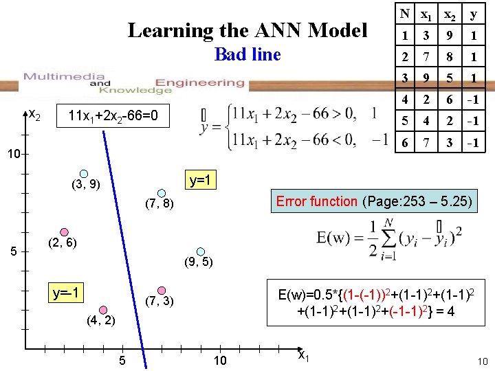
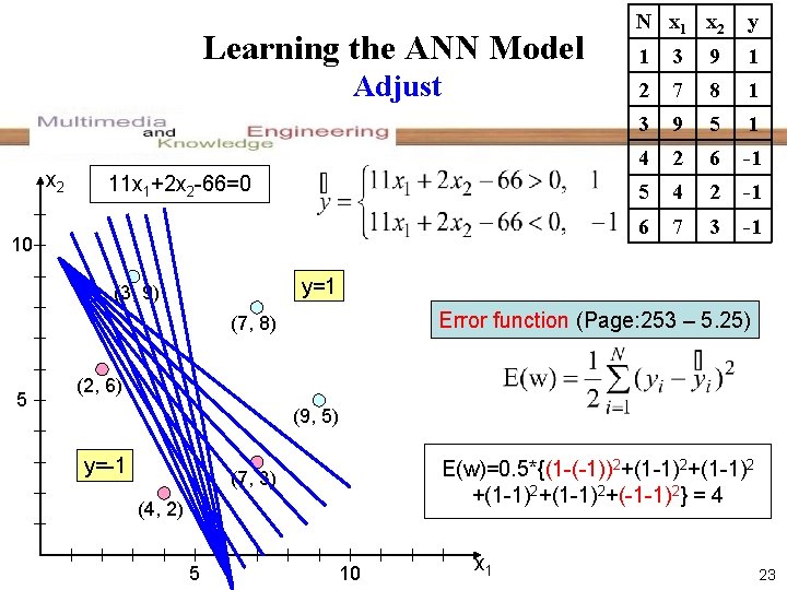
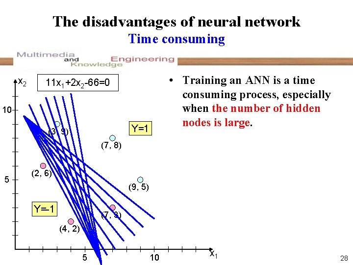
Learning the ANN Model Bad line x 2 11 x 1+2 x 2 -66=0 10 y 1 3 9 1 2 7 8 1 3 9 5 1 4 2 6 -1 5 4 2 -1 6 7 3 -1 y=1 (3, 9) Error function (Page: 253 – 5. 25) (7, 8) 5 N x 1 x 2 (2, 6) (9, 5) y=-1 E(w)=0. 5*{(1 -(-1))2+(1 -1)2+(-1 -1)2} = 4 (7, 3) (4, 2) 5 10 x 1 10

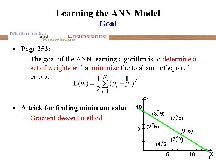
Learning the ANN Model Goal • Page 253: – The goal of the ANN learning algorithm is to determine a set of weights w that minimize the total sum of squared errors: x 2 • A trick for finding minimum value – Gradient descent method 10 (3, 9) 5 (7, 8) (2, 6) (9, 5) (4, 2) 5 (7, 3) 10 x 1 11

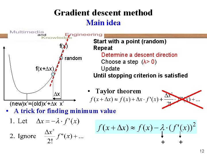
Gradient descent method Main idea f(x) random f(x+ x) x Start with a point (random) Repeat Determine a descent direction Choose a step (λ> 0) Update Until stopping criterion is satisfied • Taylor theorem (new)x’=(old)x’+ x x’ • A trick for finding minimum value + + 12

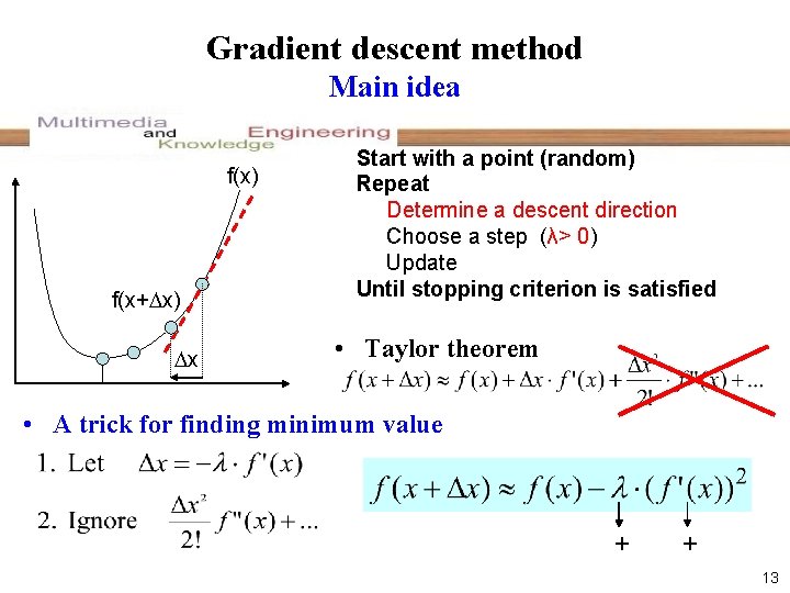
Gradient descent method Main idea f(x) f(x+ x) x Start with a point (random) Repeat Determine a descent direction Choose a step (λ> 0) Update Until stopping criterion is satisfied • Taylor theorem • A trick for finding minimum value + + 13

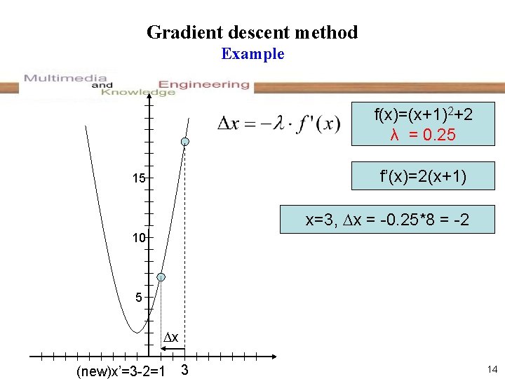
Gradient descent method Example f(x)=(x+1)2+2 λ = 0. 25 f’(x)=2(x+1) 15 x=3, x = -0. 25*8 = -2 10 5 x (new)x’=3 -2=1 3 14

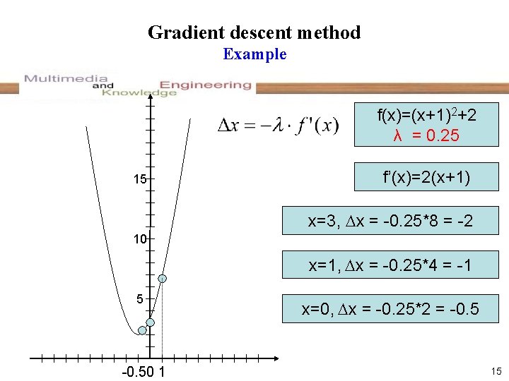
Gradient descent method Example f(x)=(x+1)2+2 λ = 0. 25 15 f’(x)=2(x+1) x=3, x = -0. 25*8 = -2 10 x=1, x = -0. 25*4 = -1 5 -0. 50 1 x=0, x = -0. 25*2 = -0. 5 15

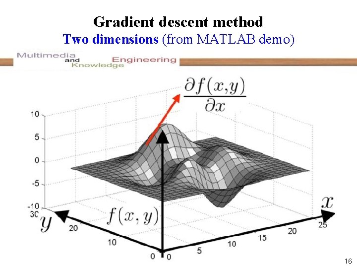
Gradient descent method Two dimensions (from MATLAB demo) 16

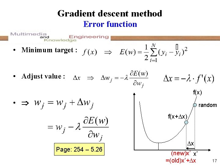
Gradient descent method Error function • Minimum target : • Adjust value : f(x) • random f(x+ x) Page: 254 – 5. 26 x (new)x’ x’ =(old)x’+ x 17

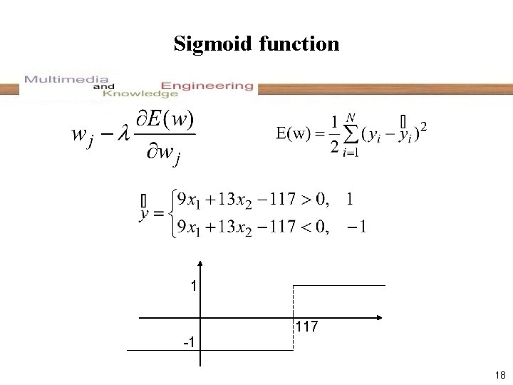
Sigmoid function 1 117 -1 18

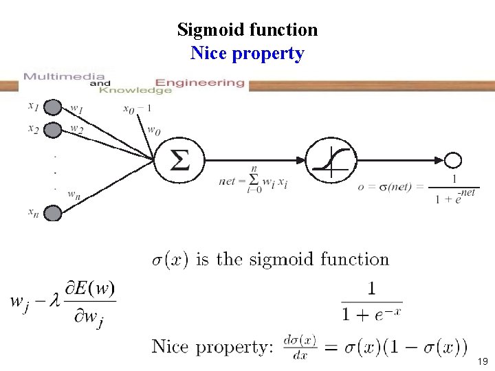
Sigmoid function Nice property 19

Derive (From Machine Learning[6]) • • For two cases • 20

Output Unit(1) (From Machine Learning[6]) • There is no direct relationship Between Ed and netj • 21

Output Unit(2) (From Machine Learning[6]) • • • 22

Learning the ANN Model Adjust x 2 11 x 1+2 x 2 -66=0 10 y 1 3 9 1 2 7 8 1 3 9 5 1 4 2 6 -1 5 4 2 -1 6 7 3 -1 y=1 (3, 9) Error function (Page: 253 – 5. 25) (7, 8) 5 N x 1 x 2 (2, 6) (9, 5) y=-1 E(w)=0. 5*{(1 -(-1))2+(1 -1)2+(-1 -1)2} = 4 (7, 3) (4, 2) 5 10 x 1 23

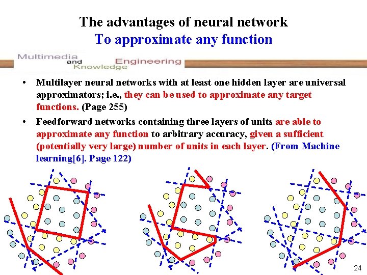
The advantages of neural network To approximate any function • Multilayer neural networks with at least one hidden layer are universal approximators; i. e. , they can be used to approximate any target functions. (Page 255) • Feedforward networks containing three layers of units are able to approximate any function to arbitrary accuracy, given a sufficient (potentially very large) number of units in each layer. (From Machine learning[6]. Page 122) 24

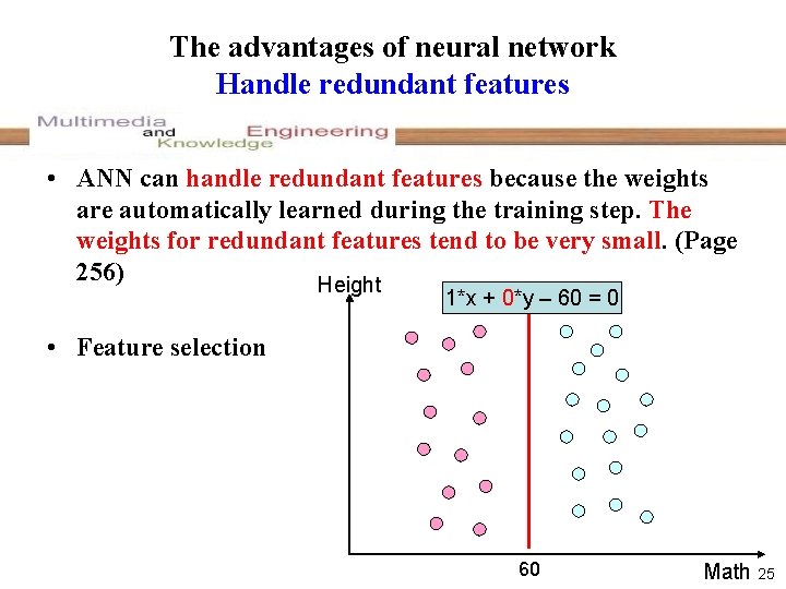
The advantages of neural network Handle redundant features • ANN can handle redundant features because the weights are automatically learned during the training step. The weights for redundant features tend to be very small. (Page 256) Height 1*x + 0*y – 60 = 0 • Feature selection 60 Math 25

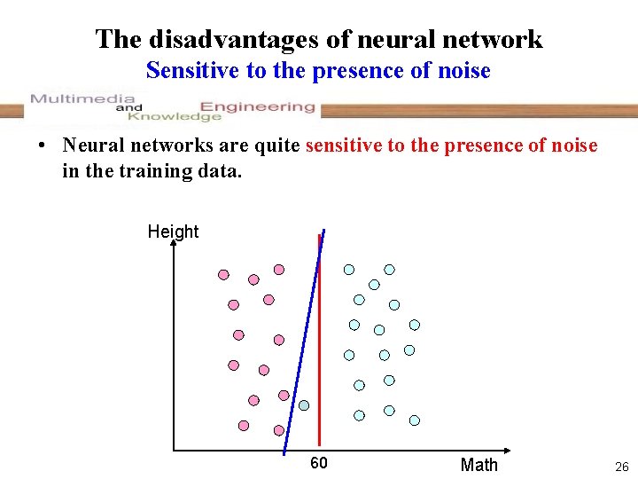
The disadvantages of neural network Sensitive to the presence of noise • Neural networks are quite sensitive to the presence of noise in the training data. Height 60 Math 26

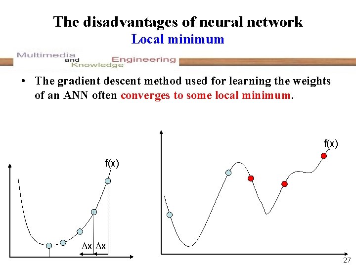
The disadvantages of neural network Local minimum • The gradient descent method used for learning the weights of an ANN often converges to some local minimum. f(x) x x 27

The disadvantages of neural network Time consuming x 2 • Training an ANN is a time consuming process, especially when the number of hidden nodes is large. 11 x 1+2 x 2 -66=0 10 Y=1 (3, 9) (7, 8) 5 (2, 6) (9, 5) Y=-1 (7, 3) (4, 2) 5 10 x 1 28

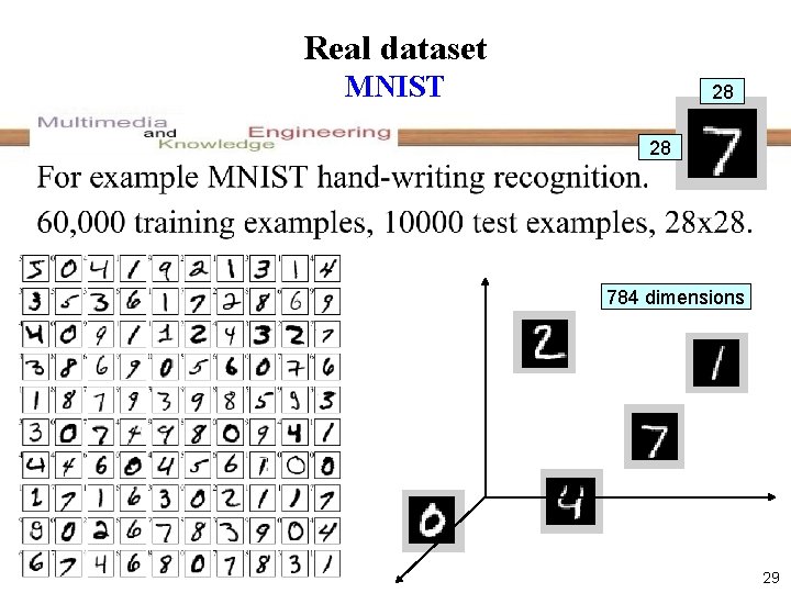
Real dataset MNIST 28 28 784 dimensions 29

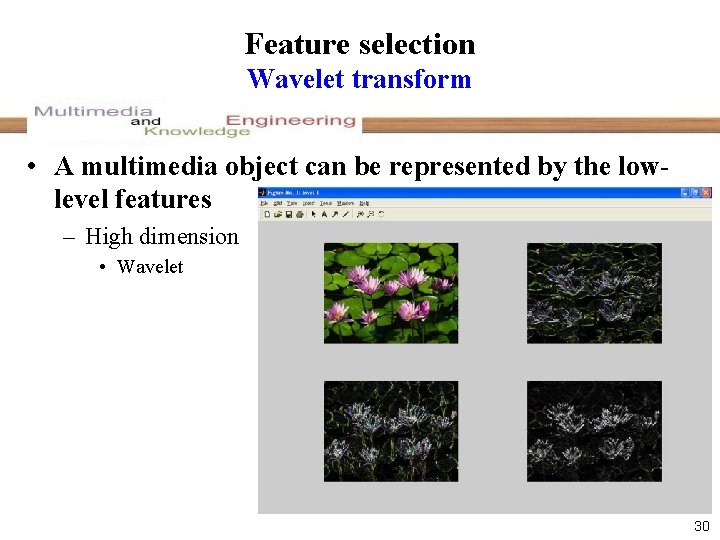
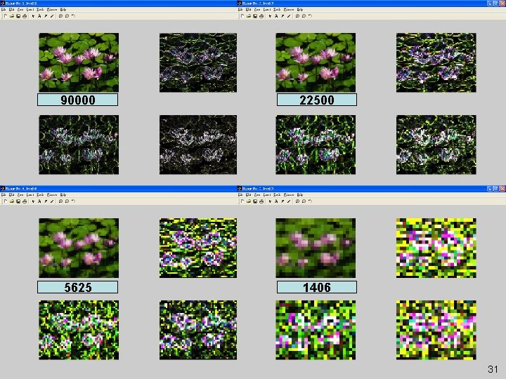
Feature selection Wavelet transform • A multimedia object can be represented by the lowlevel features – High dimension • Wavelet 30

Introduction 90000 22500 5625 1406 31

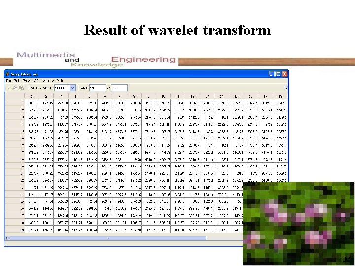
Result of wavelet transform 32

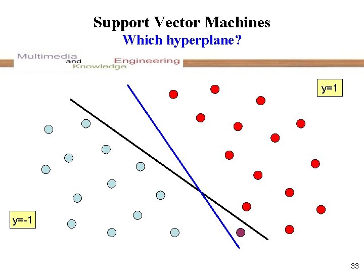
Support Vector Machines Which hyperplane? y=1 y=-1 33

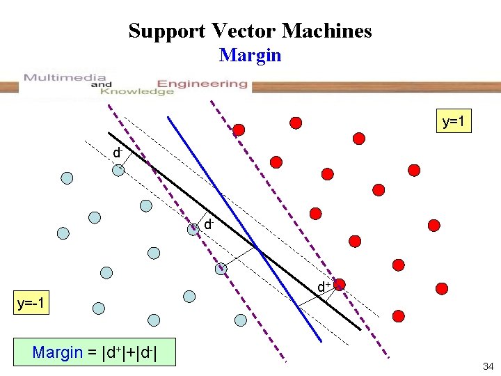
Support Vector Machines Margin y=1 d- d- d+ y=-1 Margin = |d+|+|d-| 34

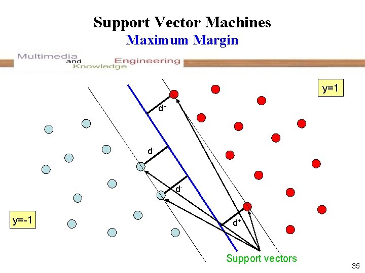
Support Vector Machines Maximum Margin y=1 d+ d- d- y=-1 d+ Support vectors 35

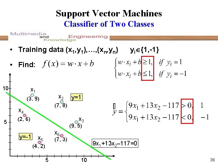
Support Vector Machines Classifier of Two Classes • Training data (x 1, y 1), …, (xn, yn) yi {1, -1} • Find: 10 x 1 x 2 (3, 9) (7, 8) x 4 5 y=1 x 3 (2, 6) (9, 5) y=-1 x 6 x 5 (7, 3) 9 x 1+13 x 2– 117=0 (4, 2) 5 10 36

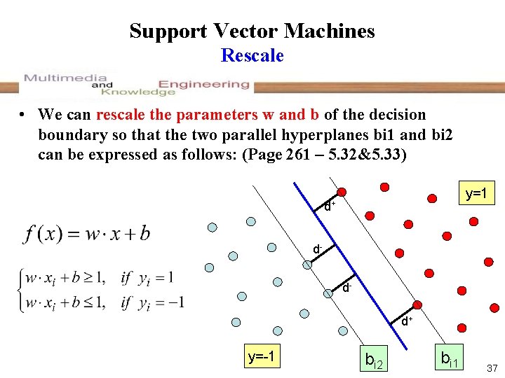
Support Vector Machines Rescale • We can rescale the parameters w and b of the decision boundary so that the two parallel hyperplanes bi 1 and bi 2 can be expressed as follows: (Page 261 – 5. 32&5. 33) y=1 d+ ddd+ y=-1 bi 2 bi 1 37

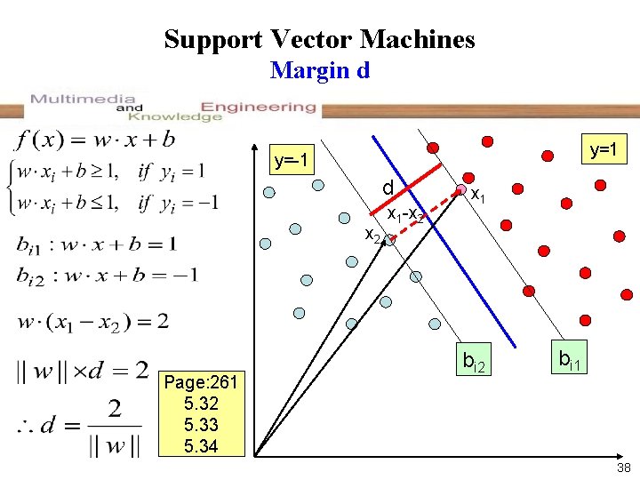
Support Vector Machines Margin d y=1 y=-1 d x 2 Page: 261 5. 32 5. 33 5. 34 x 1 -x 2 x 1 bi 2 bi 1 38

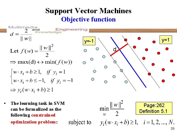
Support Vector Machines Objective function y=1 y=-1 d • The learning task in SVM can be formalized as the following constrained optimization problem: Page: 262 Definition 5. 1 39

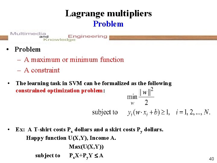
Lagrange multipliers Problem • Problem – A maximum or minimum function – A constraint • The learning task in SVM can be formalized as the following constrained optimization problem: • Ex: A T-shirt costs Px dollars and a skirt costs Py dollars. Happy function U(X, Y), Income A. Max(U(X, Y)) subject to Px. X+Py. Y A 40

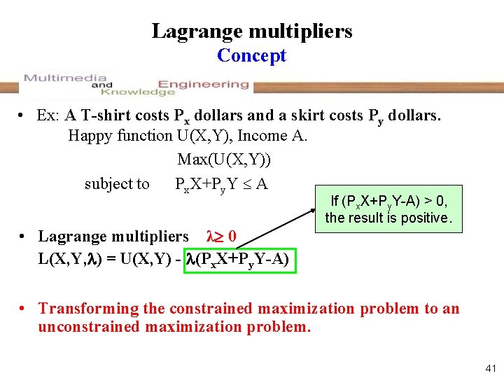
Lagrange multipliers Concept • Ex: A T-shirt costs Px dollars and a skirt costs Py dollars. Happy function U(X, Y), Income A. Max(U(X, Y)) subject to Px. X+Py. Y A If (Px. X+Py. Y-A) > 0, the result is positive. • Lagrange multipliers λ 0 L(X, Y, ) = U(X, Y) - (Px. X+Py. Y-A) • Transforming the constrained maximization problem to an unconstrained maximization problem. 41

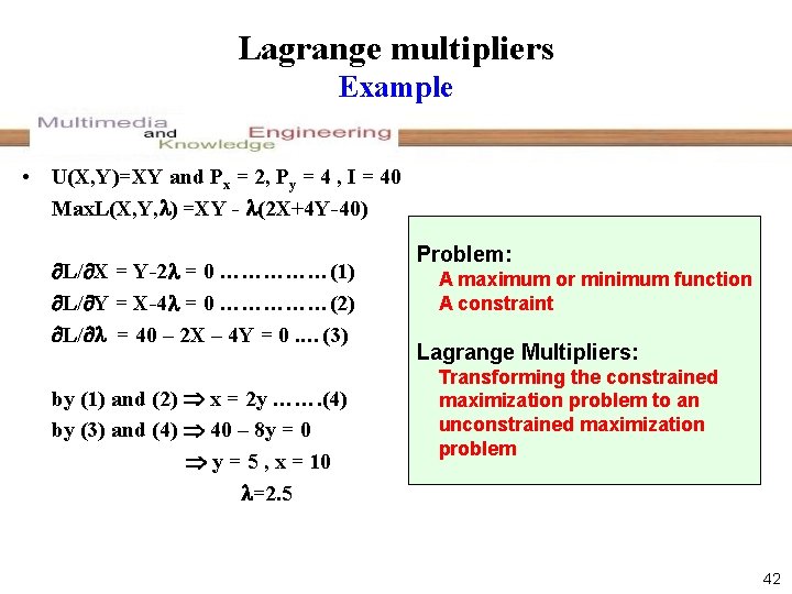
Lagrange multipliers Example • U(X, Y)=XY and Px = 2, Py = 4 , I = 40 Max. L(X, Y, ) =XY - (2 X+4 Y-40) L/ X = Y-2 = 0 ……………(1) L/ Y = X-4 = 0 ……………(2) L/ = 40 – 2 X – 4 Y = 0. …(3) by (1) and (2) x = 2 y ……. (4) by (3) and (4) 40 – 8 y = 0 y = 5 , x = 10 =2. 5 Problem: A maximum or minimum function A constraint Lagrange Multipliers: Transforming the constrained maximization problem to an unconstrained maximization problem 42

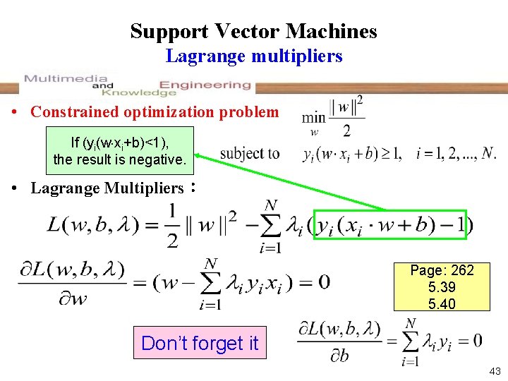
Support Vector Machines Lagrange multipliers • Constrained optimization problem If (yi(w xi+b)<1), the result is negative. • Lagrange Multipliers： Page: 262 5. 39 5. 40 Don’t forget it 43

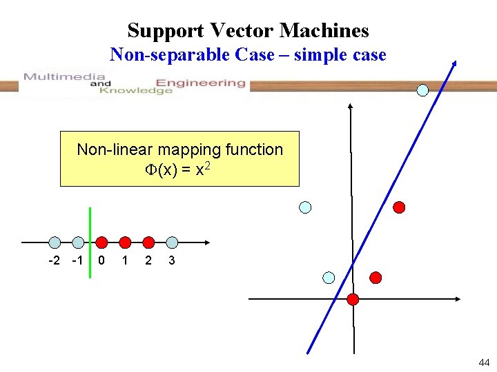
Support Vector Machines Non-separable Case – simple case Non-linear mapping function (x) = x 2 -2 -1 0 1 2 3 44

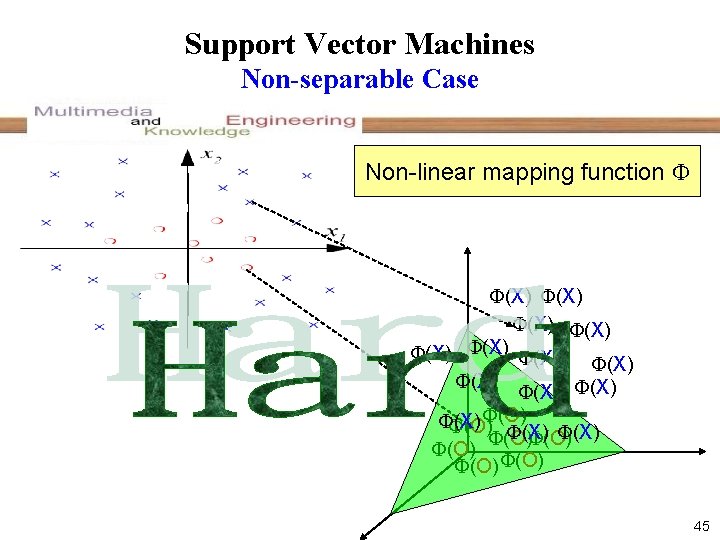
Support Vector Machines Non-separable Case Non-linear mapping function (X) (X) (X) (O) (X) (O) (O) (O) 45

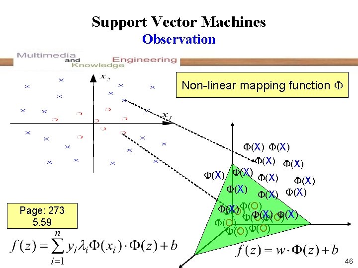
Support Vector Machines Observation Non-linear mapping function Page: 273 5. 59 (X) (X) (X) (O) (X) (O) (O) (O) 46

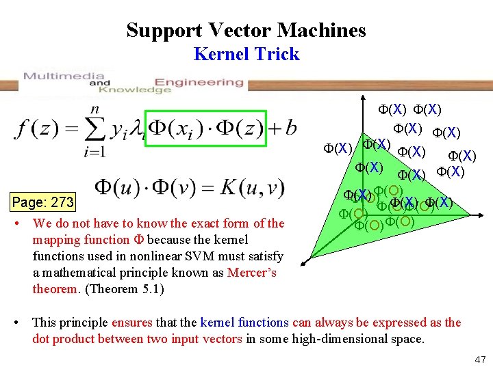
Support Vector Machines Kernel Trick Page: 273 • We do not have to know the exact form of the mapping function because the kernel functions used in nonlinear SVM must satisfy a mathematical principle known as Mercer’s theorem. (Theorem 5. 1) (X) (X) (X) (O) (X) (O) (O) (O) • This principle ensures that the kernel functions can always be expressed as the dot product between two input vectors in some high-dimensional space. 47

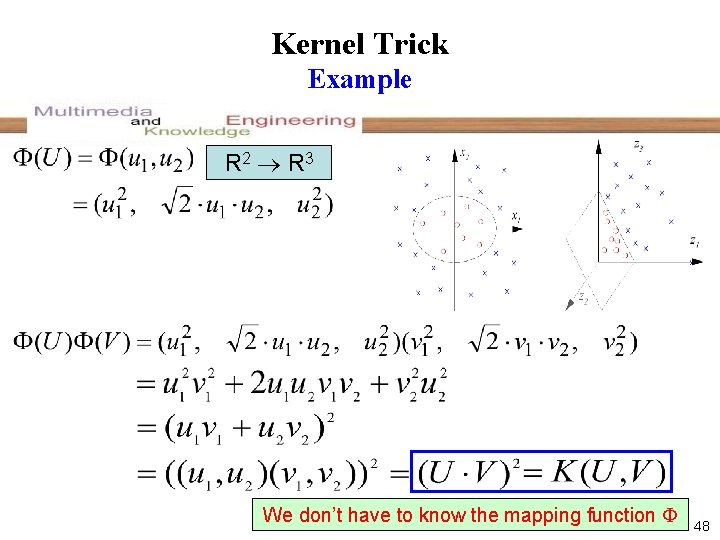
Kernel Trick Example R 2 R 3 We don’t have to know the mapping function 48

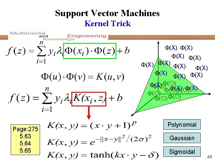
Support Vector Machines Kernel Trick (X) (X) (X) (O) (X) (O) (O) (O) Page: 275 5. 63 5. 64 5. 65 Polynomial Gaussian Sigmoidal 49

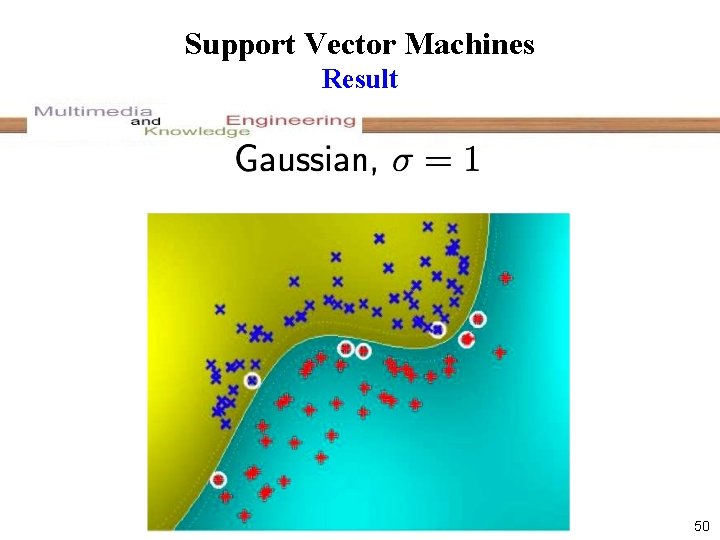
Support Vector Machines Result 50

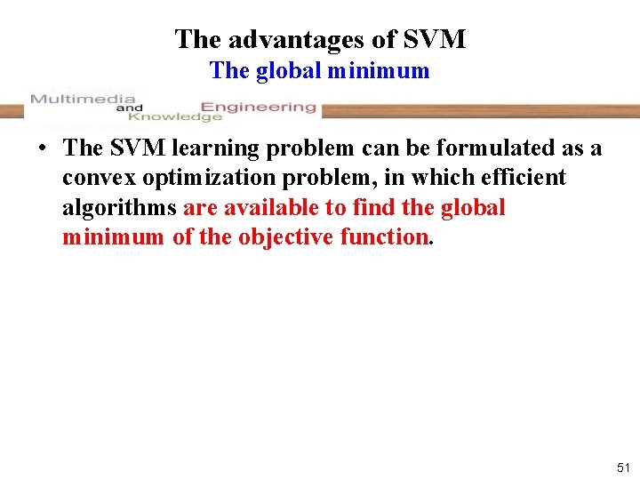
The advantages of SVM The global minimum • The SVM learning problem can be formulated as a convex optimization problem, in which efficient algorithms are available to find the global minimum of the objective function. 51

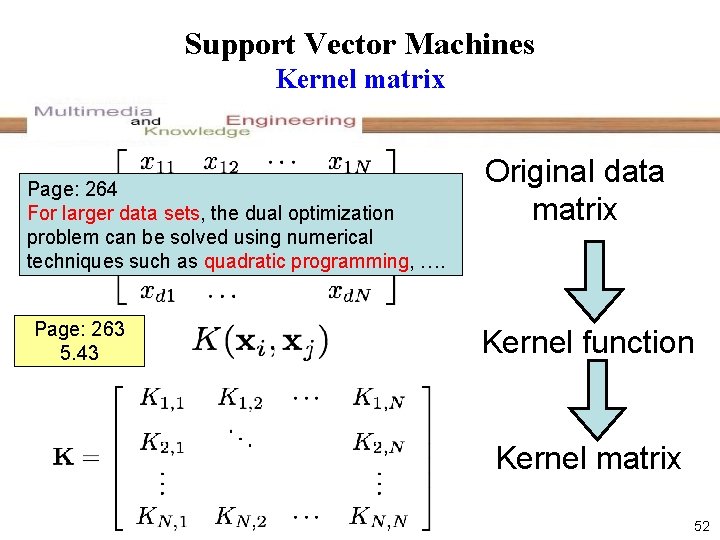
Support Vector Machines Kernel matrix Page: 264 For larger data sets, the dual optimization problem can be solved using numerical techniques such as quadratic programming, …. Page: 263 5. 43 Original data matrix Kernel function Kernel matrix 52

The disadvantages of SVM 53

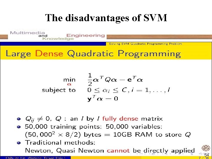
The disadvantages of SVM 54

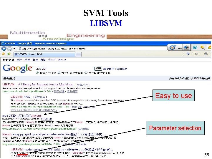
SVM Tools LIBSVM Easy to use Parameter selection 55

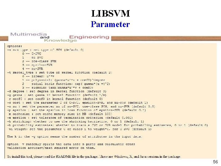
LIBSVM Parameter 56

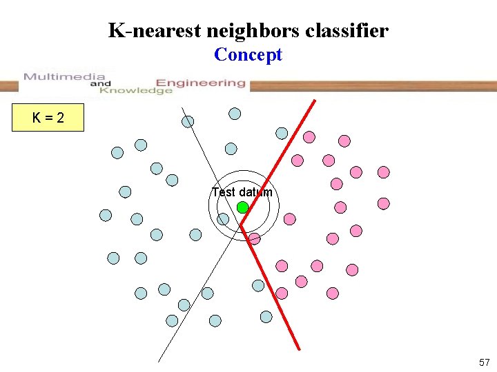
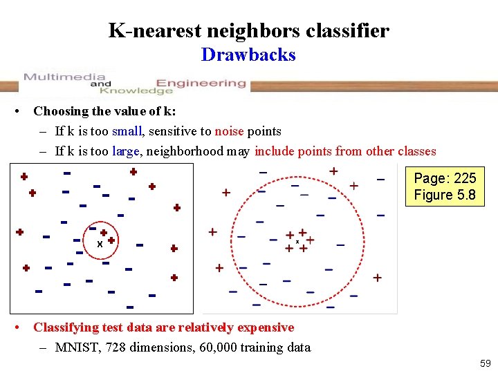
K-nearest neighbors classifier Concept K=2 1 Test datum 57

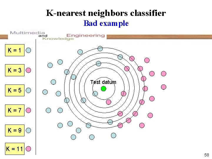
K-nearest neighbors classifier Bad example K=1 K=3 Test datum K=5 K=7 K=9 K = 11 58

K-nearest neighbors classifier Drawbacks • Choosing the value of k: – If k is too small, sensitive to noise points – If k is too large, neighborhood may include points from other classes Page: 225 Figure 5. 8 X • Classifying test data are relatively expensive – MNIST, 728 dimensions, 60, 000 training data 59

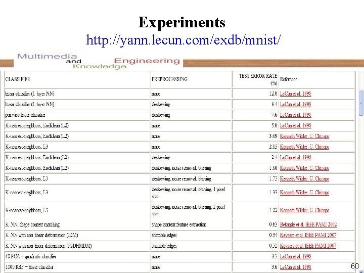
Experiments http: //yann. lecun. com/exdb/mnist/ 60

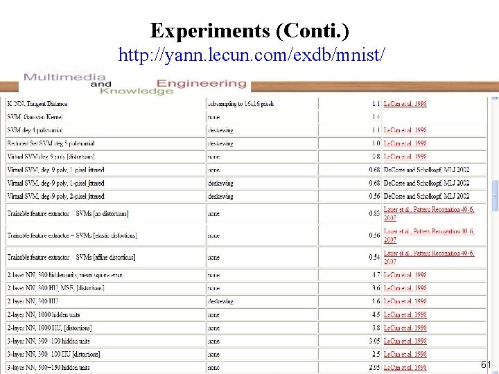
Experiments (Conti. ) http: //yann. lecun. com/exdb/mnist/ 61

Reference Basic idea of SVM (1) [1] A Training Algorithm for Optimal Margin Classifiers Bernhard E. Boser, Isabelle Guyon, Vladimir Vapnik Proceedings of the Fifth Annual ACM Conference on Computational Learning Theory, 1992, pp. 144 -152. [2] Support-Vector Networks Corinna Cortes, Vladimir Vapnik Machine Learning 20(3), 1995, pp. 273 -297. [3] A Tutorial on Support Vector Machines for Pattern Recognition Christopher J. C. Burges Data Mining and Knowledge Discovery 2(2), 1998, pp. 121 -167. 62

Reference Basic idea of SVM (2) [4] An Introduction to Kernel-Based Learning Algorithms K. -R. Müller, S. Mika, G. Rätsch, K. Tsuda, and B. Schölkopf IEEE Transactions on Neural Networks 12(2), 2001, pp 181 -202. [5] A Tutorial on Support Vector Regression A. J. Smola and B. Schölkopf Neuro. COLT Technical Report NC-TR-98 -030, Royal Holloway College, University of London, UK, 1998. [6] Machine Learning Tom M. MITCHELL Mc. GRAW-HILL International editions 63

Reference Web site • [9] LIBSVM Chih-Chung Chang and Chih-Jen Lin http: //www. csie. ntu. edu. tw/~cjlin/libsvm/ • [10] Convex Optimization with Engineering Applications Professor Stephen Boyd, Stanford University http: //www. stanford. edu/class/ee 364/ • [11] Advanced Topics in Learning & Decision Making Professor Michael I. Jordan, University of California at Berkeley http: //www. cs. berkeley. edu/~jordan/ 64