Chapter 8 Reasoning Under Uncertainty Part II Main

Chapter 8 Reasoning Under Uncertainty – Part II Main Textbook: Artificial Intelligence Foundations of Computational Agents, 2 nd Edition, David L. Poole and Alan K Mackworth, Cambridge University Press, 2018. Reference Textbook: Artificial Intelligence: A Guide to Intelligence Systems, Michael Negnevitsky, 3 rd Edition, 2011, Addison Wesley, ISBN 978 -1408225745 Asst. Prof. Dr. Anilkumar K. G 1

Probabilistic Inference • The most common probabilistic inference task is to compute the posterior distribution of a query variable or variables given some evidence. • The main approaches for probabilistic inference in belief networks are • Exact inference: • where the probabilities are computed exactly. • A simple way is to enumerate the worlds that are consistent with the evidence. • The variable elimination algorithm is an exact algorithm that uses dynamic programming and exploits conditional independence. Asst. Prof. Dr. Anilkumar K. G 2

Probabilistic Inference • Approximate inference where probabilities are only approximated and: – They produce guaranteed bounds on the probabilities. – They produce probabilistic bounds on the error produced. Such algorithms might guarantee that the error, for example, is within 0. 1 of the correct answer 95% of the time. • Variational inference, is to find an approximation to the problem that is easy to compute – First choose a class of representations that are easy to compute. This class could be a set of disconnected belief networks (with no arcs) – Next try to find a member of the class that is closest to the original problem. Thus, the problem reduces to an optimization problem of minimizing the error, followed by a simple inference problem. Asst. Prof. Dr. Anilkumar K. G 3

Variable Elimination for Belief Networks • The variable elimination (VE) algorithm, as used for finding solutions to CSPs can be adapted to find the posterior distribution for a variable in a belief network with conjunctive evidence. – The VE algorithm is based on the notion that a belief network specifies a factorization of the joint probability distribution • Recall that P(X|Y) is a function from variables (or sets of variables) X and Y into the real numbers that, given a value for X and a value for Y, returns the conditional probability of the value for X, given the value for Y. – A function of variables is called a factor. – The VE algorithm for belief networks manipulates factors to compute posterior probabilities. Asst. Prof. Dr. Anilkumar K. G 4

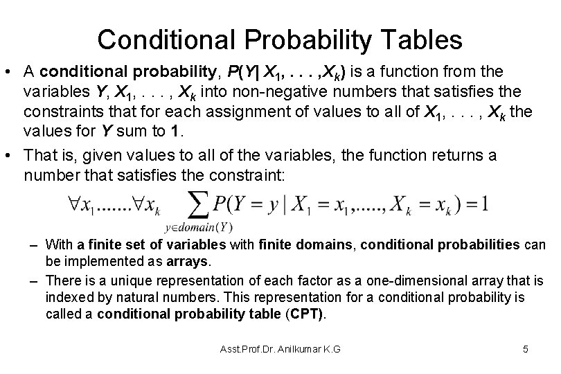
Conditional Probability Tables • A conditional probability, P(Y| X 1, . . . , Xk) is a function from the variables Y, X 1, . . . , Xk into non-negative numbers that satisfies the constraints that for each assignment of values to all of X 1, . . . , Xk the values for Y sum to 1. • That is, given values to all of the variables, the function returns a number that satisfies the constraint: – With a finite set of variables with finite domains, conditional probabilities can be implemented as arrays. – There is a unique representation of each factor as a one-dimensional array that is indexed by natural numbers. This representation for a conditional probability is called a conditional probability table (CPT). Asst. Prof. Dr. Anilkumar K. G 5

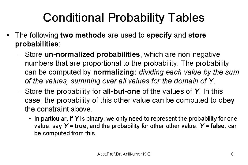
Conditional Probability Tables • The following two methods are used to specify and store probabilities: – Store un-normalized probabilities, which are non-negative numbers that are proportional to the probability. The probability can be computed by normalizing: dividing each value by the sum of the values, summing over all values for the domain of Y. – Store the probability for all-but-one of the values of Y. In this case, the probability of this other value can be computed to obey the constraint above. • In particular, if Y is binary, we only need to represent the probability for one value, say Y = true, and the probability for other value, Y = false, can be computed from this. Asst. Prof. Dr. Anilkumar K. G 6

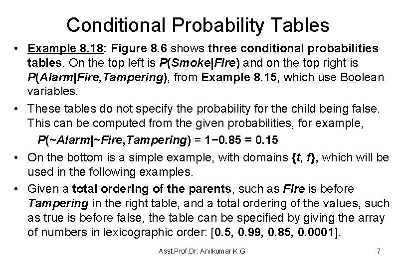
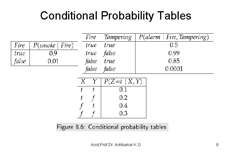
Conditional Probability Tables • Example 8. 18: Figure 8. 6 shows three conditional probabilities tables. On the top left is P(Smoke|Fire) and on the top right is P(Alarm|Fire, Tampering), from Example 8. 15, which use Boolean variables. • These tables do not specify the probability for the child being false. This can be computed from the given probabilities, for example, P(~Alarm|~Fire, Tampering) = 1− 0. 85 = 0. 15 • On the bottom is a simple example, with domains {t, f}, which will be used in the following examples. • Given a total ordering of the parents, such as Fire is before Tampering in the right table, and a total ordering of the values, such as true is before false, the table can be specified by giving the array of numbers in lexicographic order: [0. 5, 0. 99, 0. 85, 0. 0001]. Asst. Prof. Dr. Anilkumar K. G 7

Conditional Probability Tables Asst. Prof. Dr. Anilkumar K. G 8

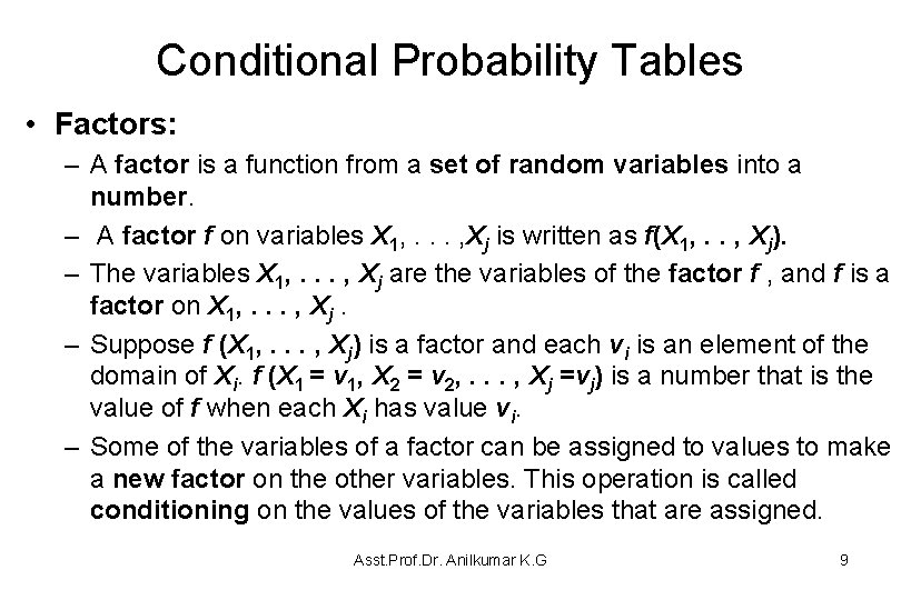
Conditional Probability Tables • Factors: – A factor is a function from a set of random variables into a number. – A factor f on variables X 1, . . . , Xj is written as f(X 1, . . , Xj). – The variables X 1, . . . , Xj are the variables of the factor f , and f is a factor on X 1, . . . , Xj. – Suppose f (X 1, . . . , Xj) is a factor and each vi is an element of the domain of Xi. f (X 1 = v 1, X 2 = v 2, . . . , Xj =vj) is a number that is the value of f when each Xi has value vi. – Some of the variables of a factor can be assigned to values to make a new factor on the other variables. This operation is called conditioning on the values of the variables that are assigned. Asst. Prof. Dr. Anilkumar K. G 9

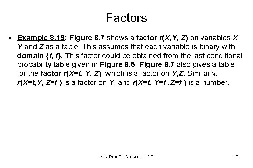
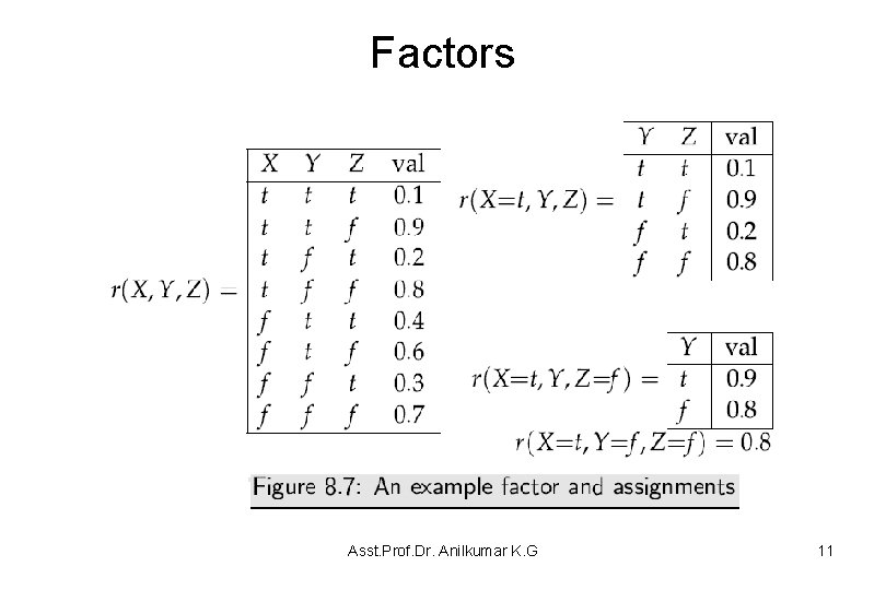
Factors • Example 8. 19: Figure 8. 7 shows a factor r(X, Y, Z) on variables X, Y and Z as a table. This assumes that each variable is binary with domain {t, f}. This factor could be obtained from the last conditional probability table given in Figure 8. 6. Figure 8. 7 also gives a table for the factor r(X=t, Y, Z), which is a factor on Y, Z. Similarly, r(X=t, Y, Z=f ) is a factor on Y, and r(X=t, Y=f , Z=f ) is a number. Asst. Prof. Dr. Anilkumar K. G 10

Factors Asst. Prof. Dr. Anilkumar K. G 11

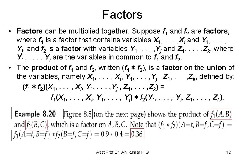
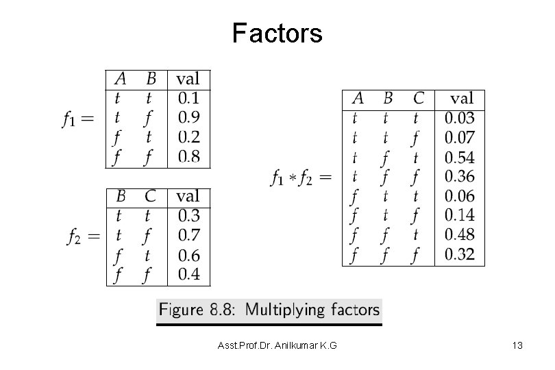
Factors • Factors can be multiplied together. Suppose f 1 and f 2 are factors, where f 1 is a factor that contains variables X 1, . . . , Xi and Y 1, . . . , Yj, and f 2 is a factor with variables Y 1, . . . , Yj and Z 1, . . . , Zk, where Y 1, . . . , Yj are the variables in common to f 1 and f 2. • The product of f 1 and f 2, written (f 1 ∗ f 2), is a factor on the union of the variables, namely X 1, . . . , Xi, Y 1, . . . , Yj , Z 1, . . . , Zk, defined by: (f 1 ∗ f 2)(X 1, . . . , Xi, Y 1, . . . , Yj , Z 1, . . . , Zk) = f 1(X 1, . . . , Xi, Y 1, . . . , Yj) ∗ f 2(Y 1, . . . , Yj, Z 1, . . . , Zk). Asst. Prof. Dr. Anilkumar K. G 12

Factors Asst. Prof. Dr. Anilkumar K. G 13

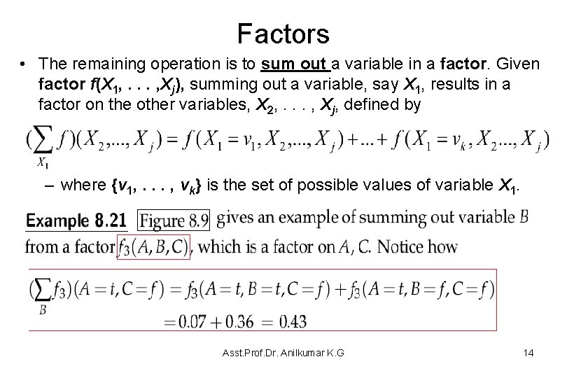
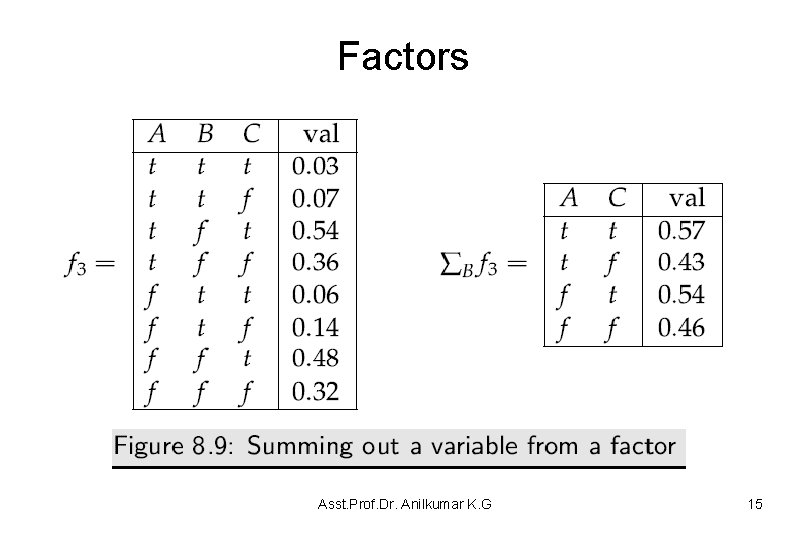
Factors • The remaining operation is to sum out a variable in a factor. Given factor f(X 1, . . . , Xj), summing out a variable, say X 1, results in a factor on the other variables, X 2, . . . , Xj, defined by – where {v 1, . . . , vk} is the set of possible values of variable X 1. Asst. Prof. Dr. Anilkumar K. G 14

Factors Asst. Prof. Dr. Anilkumar K. G 15

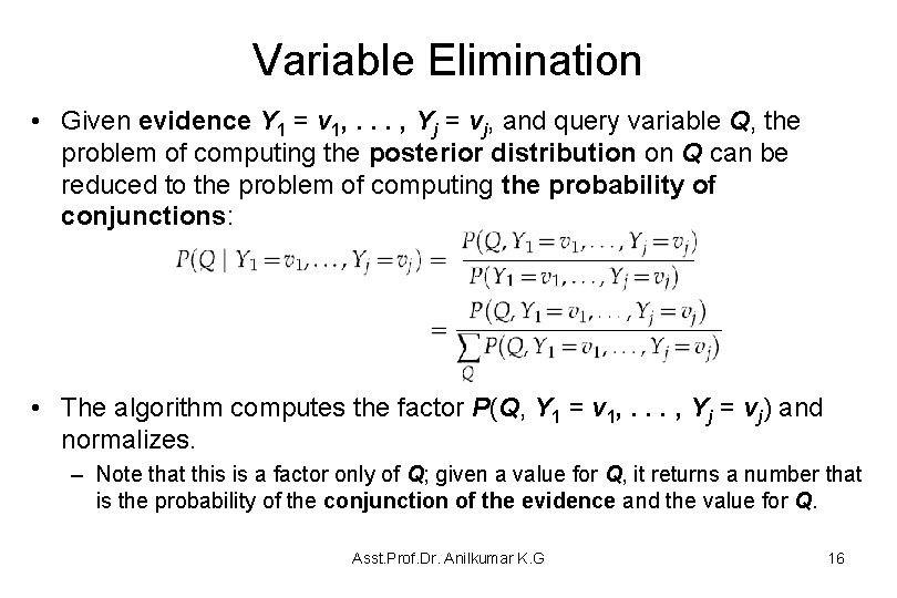
Variable Elimination • Given evidence Y 1 = v 1, . . . , Yj = vj, and query variable Q, the problem of computing the posterior distribution on Q can be reduced to the problem of computing the probability of conjunctions: • The algorithm computes the factor P(Q, Y 1 = v 1, . . . , Yj = vj) and normalizes. – Note that this is a factor only of Q; given a value for Q, it returns a number that is the probability of the conjunction of the evidence and the value for Q. Asst. Prof. Dr. Anilkumar K. G 16

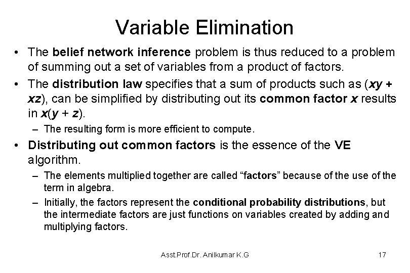
Variable Elimination • The belief network inference problem is thus reduced to a problem of summing out a set of variables from a product of factors. • The distribution law specifies that a sum of products such as (xy + xz), can be simplified by distributing out its common factor x results in x(y + z). – The resulting form is more efficient to compute. • Distributing out common factors is the essence of the VE algorithm. – The elements multiplied together are called “factors” because of the term in algebra. – Initially, the factors represent the conditional probability distributions, but the intermediate factors are just functions on variables created by adding and multiplying factors. Asst. Prof. Dr. Anilkumar K. G 17

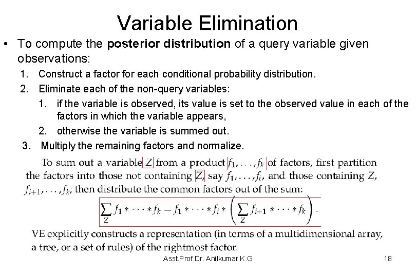
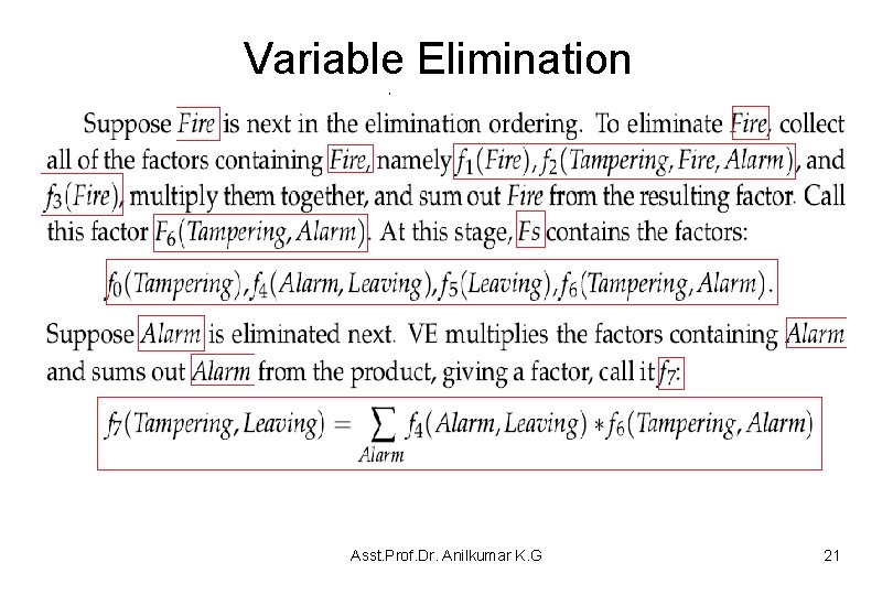
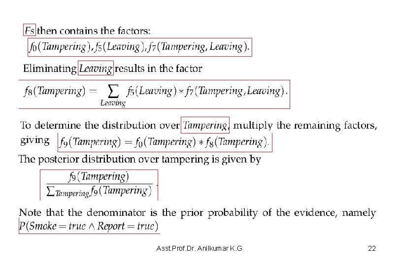
Variable Elimination • To compute the posterior distribution of a query variable given observations: 1. Construct a factor for each conditional probability distribution. 2. Eliminate each of the non-query variables: 1. if the variable is observed, its value is set to the observed value in each of the factors in which the variable appears, 2. otherwise the variable is summed out. 3. Multiply the remaining factors and normalize. Asst. Prof. Dr. Anilkumar K. G 18

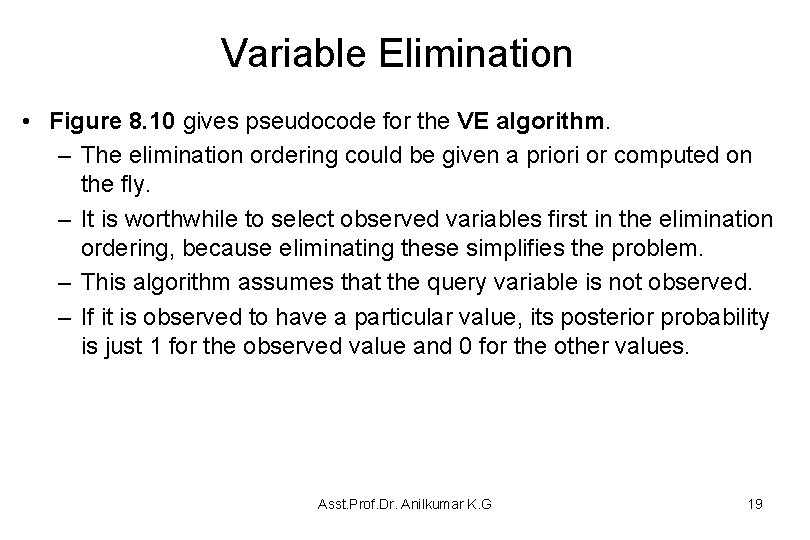
Variable Elimination • Figure 8. 10 gives pseudocode for the VE algorithm. – The elimination ordering could be given a priori or computed on the fly. – It is worthwhile to select observed variables first in the elimination ordering, because eliminating these simplifies the problem. – This algorithm assumes that the query variable is not observed. – If it is observed to have a particular value, its posterior probability is just 1 for the observed value and 0 for the other values. Asst. Prof. Dr. Anilkumar K. G 19

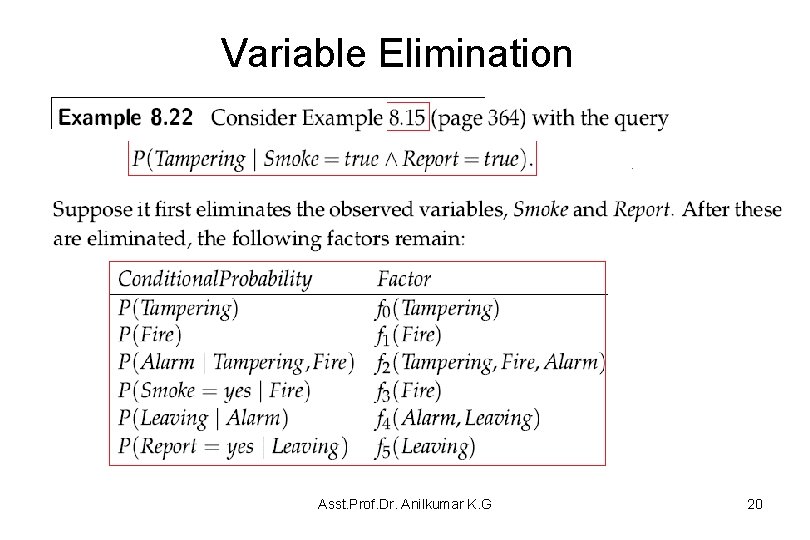
Variable Elimination Asst. Prof. Dr. Anilkumar K. G 20

Variable Elimination Asst. Prof. Dr. Anilkumar K. G 21

Asst. Prof. Dr. Anilkumar K. G 22

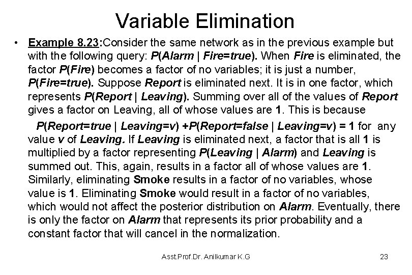
Variable Elimination • Example 8. 23: Consider the same network as in the previous example but with the following query: P(Alarm | Fire=true). When Fire is eliminated, the factor P(Fire) becomes a factor of no variables; it is just a number, P(Fire=true). Suppose Report is eliminated next. It is in one factor, which represents P(Report | Leaving). Summing over all of the values of Report gives a factor on Leaving, all of whose values are 1. This is because P(Report=true | Leaving=v) +P(Report=false | Leaving=v) = 1 for any value v of Leaving. If Leaving is eliminated next, a factor that is all 1 is multiplied by a factor representing P(Leaving | Alarm) and Leaving is summed out. This, again, results in a factor all of whose values are 1. Similarly, eliminating Smoke results in a factor of no variables, whose value is 1. Eliminating Smoke would result in a factor of no variables, which would not affect the posterior distribution on Alarm. Eventually, there is only the factor on Alarm that represents its prior probability and a constant factor that will cancel in the normalization. Asst. Prof. Dr. Anilkumar K. G 23

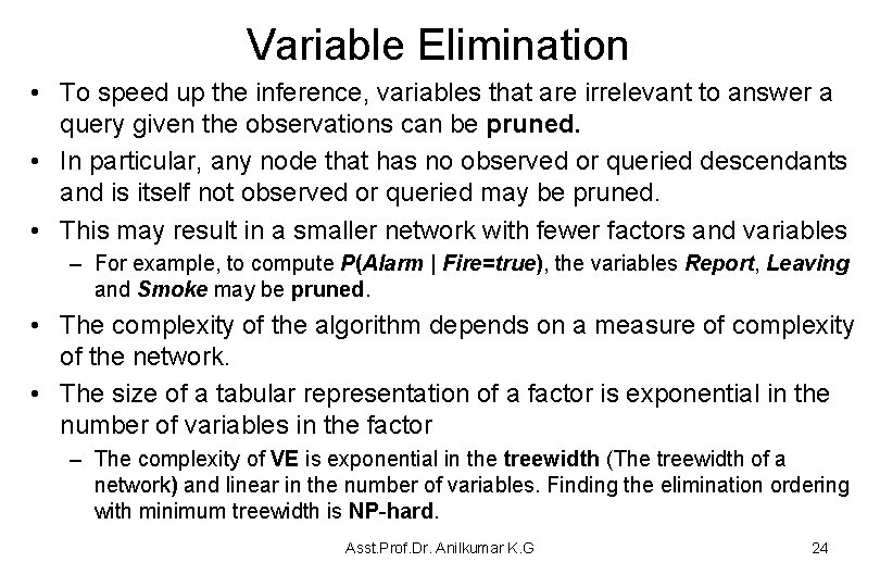
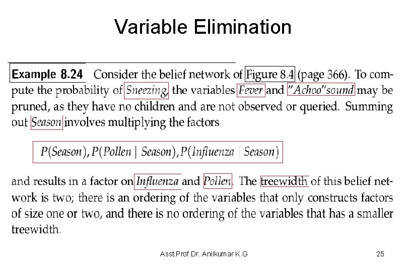
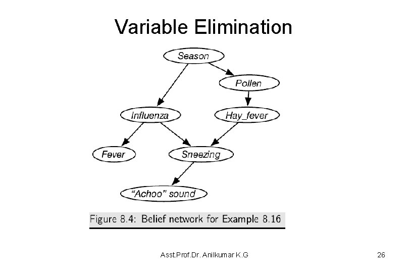
Variable Elimination • To speed up the inference, variables that are irrelevant to answer a query given the observations can be pruned. • In particular, any node that has no observed or queried descendants and is itself not observed or queried may be pruned. • This may result in a smaller network with fewer factors and variables – For example, to compute P(Alarm | Fire=true), the variables Report, Leaving and Smoke may be pruned. • The complexity of the algorithm depends on a measure of complexity of the network. • The size of a tabular representation of a factor is exponential in the number of variables in the factor – The complexity of VE is exponential in the treewidth (The treewidth of a network) and linear in the number of variables. Finding the elimination ordering with minimum treewidth is NP-hard. Asst. Prof. Dr. Anilkumar K. G 24

Variable Elimination Asst. Prof. Dr. Anilkumar K. G 25

Variable Elimination Asst. Prof. Dr. Anilkumar K. G 26

Representing Conditional Probabilities and Factors • This section explores some variants for representing factors and conditional probabilities. • A conditional probability distribution is a function on variables; given an assignment to the values of the variables, it gives a number. • A factor is a function of a set of variables; the variables it depends on are the scope of the factor. • Thus a conditional probability is a factor, as it is a function on variables. • Some of the representations are for arbitrary factors and some are specific to conditional probabilities. Asst. Prof. Dr. Anilkumar K. G 27

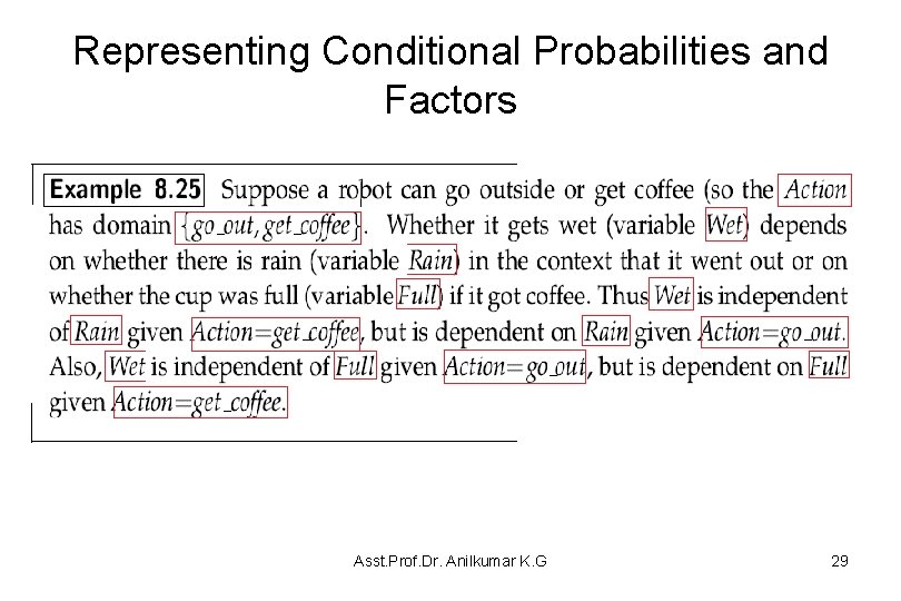
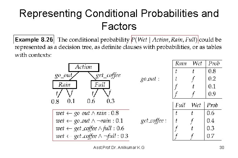
Representing Conditional Probabilities and Factors • Factors do not have to be implemented as conditional probability tables. • The resulting tabular representation is often too large when there are many parents. • Often, structure in conditional probabilities can be exploited. • One such structure exploits context-specific independence, where one variable is conditionally independent of another, given a particular value of the third variable. Asst. Prof. Dr. Anilkumar K. G 28

Representing Conditional Probabilities and Factors Asst. Prof. Dr. Anilkumar K. G 29

Representing Conditional Probabilities and Factors Asst. Prof. Dr. Anilkumar K. G 30

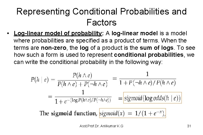
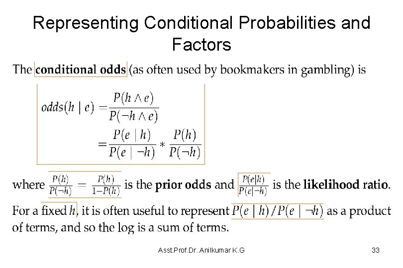
Representing Conditional Probabilities and Factors • Log-linear model of probability: A log-linear model is a model where probabilities are specified as a product of terms. When the terms are non-zero, the log of a product is the sum of logs. To see how such a form is used to represent conditional probabilities, we can write the conditional probability in the following way: Asst. Prof. Dr. Anilkumar K. G 31

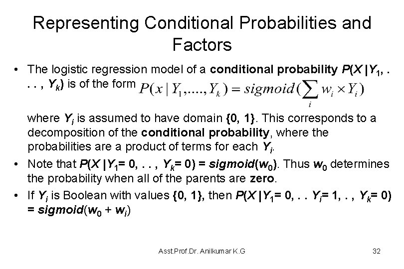
Representing Conditional Probabilities and Factors • The logistic regression model of a conditional probability P(X |Y 1, . . . , Yk) is of the form where Yi is assumed to have domain {0, 1}. This corresponds to a decomposition of the conditional probability, where the probabilities are a product of terms for each Yi. • Note that P(X |Y 1= 0, . . , Yk= 0) = sigmoid(w 0). Thus w 0 determines the probability when all of the parents are zero. • If Yi is Boolean with values {0, 1}, then P(X |Y 1= 0, . . Yi= 1, . , Yk= 0) = sigmoid(w 0 + wi) Asst. Prof. Dr. Anilkumar K. G 32

Representing Conditional Probabilities and Factors Asst. Prof. Dr. Anilkumar K. G 33

Representing Conditional Probabilities and Factors Asst. Prof. Dr. Anilkumar K. G 34

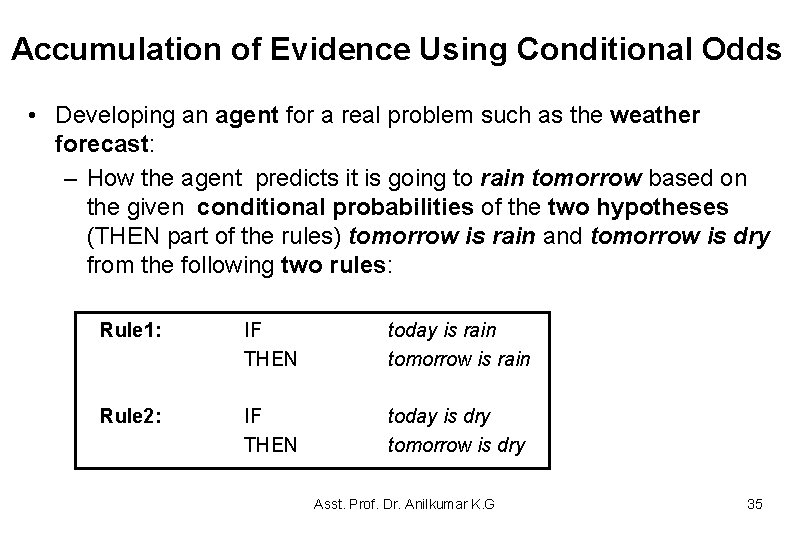
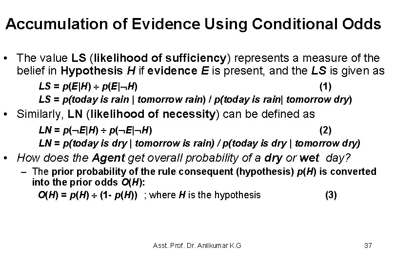
Accumulation of Evidence Using Conditional Odds • Developing an agent for a real problem such as the weather forecast: – How the agent predicts it is going to rain tomorrow based on the given conditional probabilities of the two hypotheses (THEN part of the rules) tomorrow is rain and tomorrow is dry from the following two rules: Rule 1: IF THEN today is rain tomorrow is rain Rule 2: IF THEN today is dry tomorrow is dry Asst. Prof. Dr. Anilkumar K. G 35

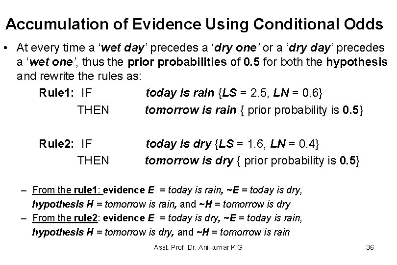
Accumulation of Evidence Using Conditional Odds • At every time a ‘wet day’ precedes a ‘dry one’ or a ‘dry day’ precedes a ‘wet one’, thus the prior probabilities of 0. 5 for both the hypothesis and rewrite the rules as: Rule 1: IF today is rain {LS = 2. 5, LN = 0. 6} THEN tomorrow is rain { prior probability is 0. 5} Rule 2: IF THEN today is dry {LS = 1. 6, LN = 0. 4} tomorrow is dry { prior probability is 0. 5} – From the rule 1: evidence E = today is rain, ~E = today is dry, hypothesis H = tomorrow is rain, and ~H = tomorrow is dry – From the rule 2: evidence E = today is dry, ~E = today is rain, hypothesis H = tomorrow is dry, and ~H = tomorrow is rain Asst. Prof. Dr. Anilkumar K. G 36

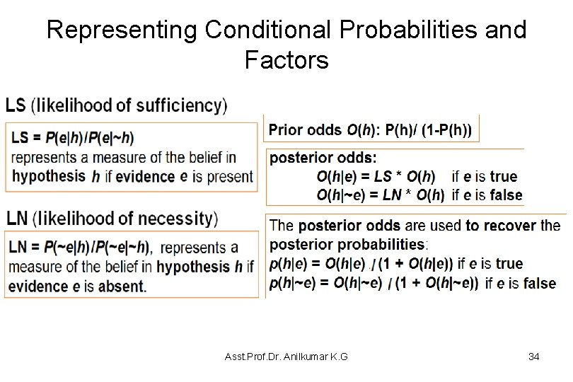
Accumulation of Evidence Using Conditional Odds • The value LS (likelihood of sufficiency) represents a measure of the belief in Hypothesis H if evidence E is present, and the LS is given as LS = p(E|H) p(E| H) (1) LS = p(today is rain | tomorrow rain) / p(today is rain| tomorrow dry) • Similarly, LN (likelihood of necessity) can be defined as LN = p( E|H) p( E| H) (2) LN = p(today is dry | tomorrow is rain) / p(today is dry | tomorrow dry) • How does the Agent get overall probability of a dry or wet day? – The prior probability of the rule consequent (hypothesis) p(H) is converted into the prior odds O(H): O(H) = p(H) (1 - p(H)) ; where H is the hypothesis (3) Asst. Prof. Dr. Anilkumar K. G 37

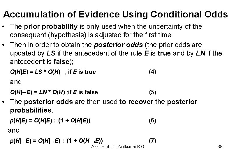
Accumulation of Evidence Using Conditional Odds • The prior probability is only used when the uncertainty of the consequent (hypothesis) is adjusted for the first time • Then in order to obtain the posterior odds (the prior odds are updated by LS if the antecedent of the rule E is true and by LN if the antecedent is false); O(H|E) = LS * O(H) ; if E is true (4) and O(H| E) = LN * O(H) ; if E is false (5) • The posterior odds are then used to recover the posterior probabilities: p(H|E) = O(H|E) (1 + O(H|E)) (6) and p(H| E) = O(H| E) (1 + O(H| E)) Asst. Prof. Dr. Anilkumar K. G (7) 38

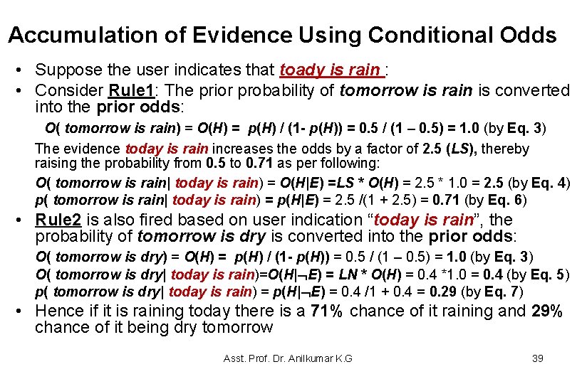
Accumulation of Evidence Using Conditional Odds • Suppose the user indicates that toady is rain : • Consider Rule 1: The prior probability of tomorrow is rain is converted into the prior odds: O( tomorrow is rain) = O(H) = p(H) / (1 - p(H)) = 0. 5 / (1 – 0. 5) = 1. 0 (by Eq. 3) The evidence today is rain increases the odds by a factor of 2. 5 (LS), thereby raising the probability from 0. 5 to 0. 71 as per following: O( tomorrow is rain| today is rain) = O(H|E) =LS * O(H) = 2. 5 * 1. 0 = 2. 5 (by Eq. 4) p( tomorrow is rain| today is rain) = p(H|E) = 2. 5 /(1 + 2. 5) = 0. 71 (by Eq. 6) • Rule 2 is also fired based on user indication “today is rain”, the probability of tomorrow is dry is converted into the prior odds: O( tomorrow is dry) = O(H) = p(H) / (1 - p(H)) = 0. 5 / (1 – 0. 5) = 1. 0 (by Eq. 3) O( tomorrow is dry| today is rain)=O(H| E) = LN * O(H) = 0. 4 *1. 0 = 0. 4 (by Eq. 5) p( tomorrow is dry| today is rain) = p(H| E) = 0. 4 /1 + 0. 4 = 0. 29 (by Eq. 7) • Hence if it is raining today there is a 71% chance of it raining and 29% chance of it being dry tomorrow Asst. Prof. Dr. Anilkumar K. G 39

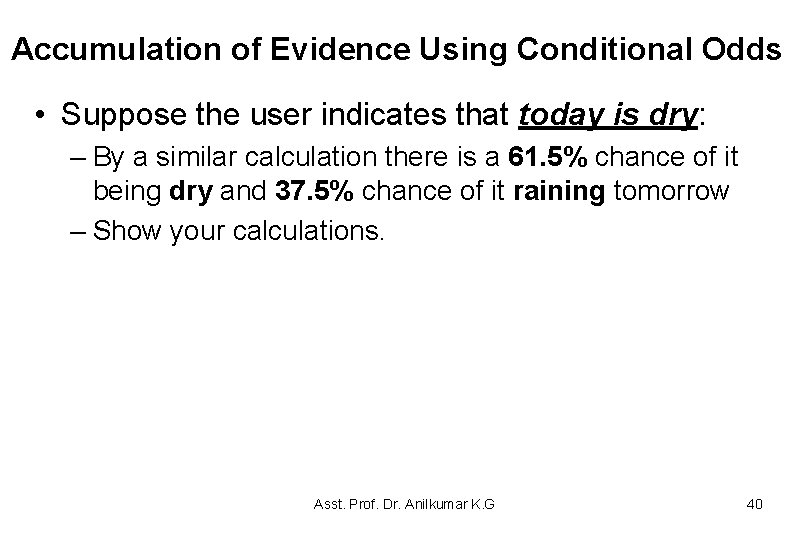
Accumulation of Evidence Using Conditional Odds • Suppose the user indicates that today is dry: – By a similar calculation there is a 61. 5% chance of it being dry and 37. 5% chance of it raining tomorrow – Show your calculations. Asst. Prof. Dr. Anilkumar K. G 40

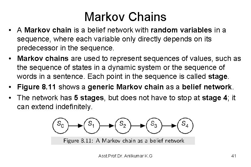
Markov Chains • A Markov chain is a belief network with random variables in a sequence, where each variable only directly depends on its predecessor in the sequence. • Markov chains are used to represent sequences of values, such as the sequence of states in a dynamic system or the sequence of words in a sentence. Each point in the sequence is called stage. • Figure 8. 11 shows a generic Markov chain as a belief network. • The network has 5 stages, but does not have to stop at stage 4; it can extend indefinitely. Asst. Prof. Dr. Anilkumar K. G 41

Markov Chains • The belief network conveys the independence assumption P(Si+1 | S 0, . . . , Si) = P(Si+1 | Si), which is called the Markov assumption. – Often the sequences are in time and, St represents the state at time t. • Intuitively, St conveys all of the information about the history that could affect the future states. – The independence assumption of the Markov chain can be seen as “the future is conditionally independent of the past given the present. ” • A Markov chain is a stationary model or time-homogenous model if the variables all have the same domain, and the transition probabilities are the same for each stage, i. e. , for all i ≥ 0, P(Si+1|Si) = P(S 1|S 0) • To specify a stationary Markov chain, two conditional probabilities are provided: – P(S 0) specifies the initial conditions – P(Si+1|Si) specifies the dynamics, which is the same for each i ≥ 0. Asst. Prof. Dr. Anilkumar K. G 42

Markov Chains https: //brilliant. org/wiki/markov-chains/ • Markov chain is a stochastic process, but it differs from a general stochastic process in that a Markov chain must be "memory-less. " – That is, (the probability of) future actions are not dependent upon the steps that led up to the present state. This is called the Markov property. – While theory of Markov chains is important precisely because so many "everyday" processes satisfy the Markov property, there are many common examples of stochastic properties that do not satisfy the Markov property. Asst. Prof. Dr. Anilkumar K. G 43

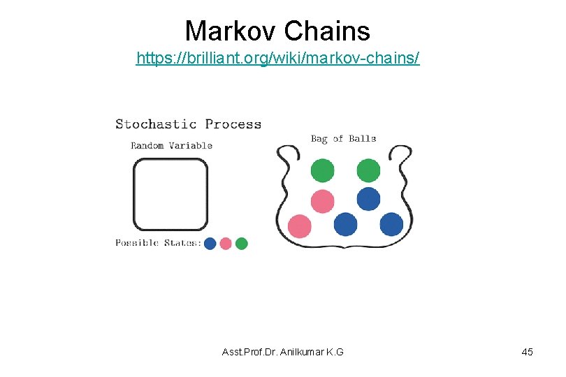
Markov Chains https: //brilliant. org/wiki/markov-chains/ • A common probability question asks what the probability of getting a certain color ball is when selecting uniformly at random from a bag of multi-colored balls. • It could also ask what the probability of the next ball is, and so on. • In such a way, a stochastic process begins to exist with color for the random variable, and it does not satisfy the Markov property. • Depending upon which balls are removed, the probability of getting a certain color ball later may be drastically different. Asst. Prof. Dr. Anilkumar K. G 44

Markov Chains https: //brilliant. org/wiki/markov-chains/ Asst. Prof. Dr. Anilkumar K. G 45

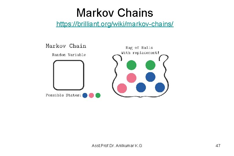
Markov Chains https: //brilliant. org/wiki/markov-chains/ • A variant of the same question asks once again for ball color, but it allows replacement each time a ball is drawn. • Once again, this creates a stochastic process with color for the random variable. • This process, however, does satisfy the Markov property. Asst. Prof. Dr. Anilkumar K. G 46

Markov Chains https: //brilliant. org/wiki/markov-chains/ Asst. Prof. Dr. Anilkumar K. G 47

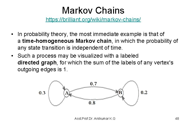
Markov Chains https: //brilliant. org/wiki/markov-chains/ • In probability theory, the most immediate example is that of a time-homogeneous Markov chain, in which the probability of any state transition is independent of time. • Such a process may be visualized with a labeled directed graph, for which the sum of the labels of any vertex's outgoing edges is 1. Asst. Prof. Dr. Anilkumar K. G 48

Markov Chains https: //brilliant. org/wiki/markov-chains/ • In order to move from A to B, the process must either stay on A the first move, then move to B the second move; or move to B the first move, then stay on B the second move. According to the diagram, the probability of that is 0. 3 x 0. 7+ 0. 7 x 0. 2 = 0. 35. • Alternatively, the probability that the process will be on A after 2 moves is 0. 3 x 0. 3 + 0. 7 x 0. 8 = 0. 65. Since there are only two states in the chain, the process must be on B if it is not on A, and therefore the probability that the process will be on B after 2 moves is 1 - 0. 65 = 0. 35. Asst. Prof. Dr. Anilkumar K. G 49