Topic 1 Measurement and uncertainties 1 2 Uncertainties

Topic 1: Measurement and uncertainties 1. 2 – Uncertainties and errors

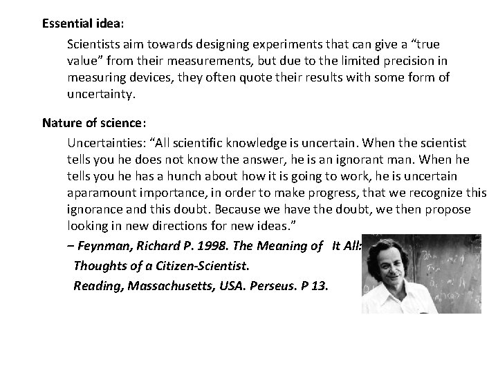
Essential idea: Scientists aim towards designing experiments that can give a “true value” from their measurements, but due to the limited precision in measuring devices, they often quote their results with some form of uncertainty. Nature of science: Uncertainties: “All scientific knowledge is uncertain. When the scientist tells you he does not know the answer, he is an ignorant man. When he tells you he has a hunch about how it is going to work, he is uncertain aparamount importance, in order to make progress, that we recognize this ignorance and this doubt. Because we have the doubt, we then propose looking in new directions for new ideas. ” – Feynman, Richard P. 1998. The Meaning of It All: Thoughts of a Citizen-Scientist. Reading, Massachusetts, USA. Perseus. P 13.

Understandings: • Random and systematic errors • Absolute, fractional and percentage uncertainties • Error bars • Uncertainty of gradients and intercepts Applications and skills: • Explaining how random and systematic errors can be identified and reduced • Collecting data that include absolute and/or fractional uncertainties and stating these as an uncertainty range (expressed as: best estimate ± uncertainty range) • Propagating uncertainties through calculations involving addition, subtraction, multiplication, division and raising to a power • Determining the uncertainty in gradients and intercepts

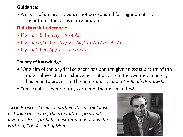
Guidance: • Analysis of uncertainties will not be expected for trigonometric or logarithmic functions in examinations Data booklet reference: • If y = a b then y = a + b • If y = a · b / c then y / y = a / a + b / b + c / c • If y = a n then y / y = | n · a / a | Theory of knowledge: • “One aim of the physical sciences has been to give an exact picture of the material world. One achievement of physics in the twentieth century has been to prove that this aim is unattainable. ” – Jacob Bronowski. • Can scientists ever be truly certain of their discoveries? Jacob Bronowski was a mathematician, biologist, historian of science, theatre author, poet and inventor. He is probably best remembered as the writer of The Ascent of Man.

Utilization: • Students studying more than one group 4 subject will be able to use these skills across all subjects Aims: • Aim 4: it is important that students see scientific errors and uncertainties not only as the range of possible answers but as an integral part of the scientific process • Aim 9: the process of using uncertainties in classical physics can be compared to the view of uncertainties in modern (and particularly quantum) physics

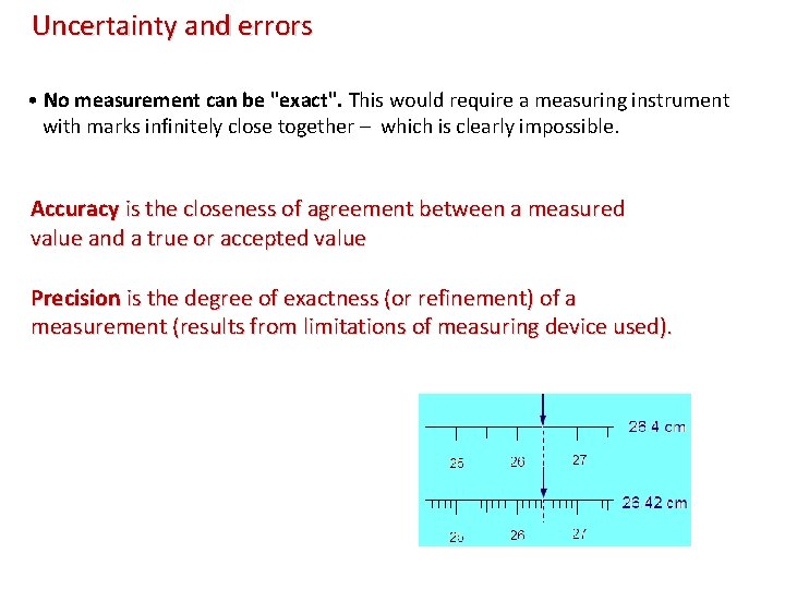
Uncertainty and errors • No measurement can be "exact". This would require a measuring instrument with marks infinitely close together – which is clearly impossible. Accuracy is the closeness of agreement between a measured value and a true or accepted value Precision is the degree of exactness (or refinement) of a measurement (results from limitations of measuring device used).

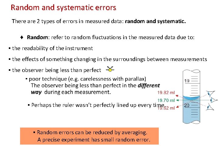
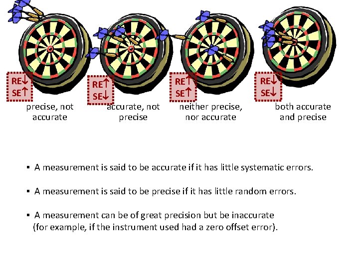
Random and systematic errors There are 2 types of errors in measured data: random and systematic. Random: refer to random fluctuations in the measured data due to: ▪ the readability of the instrument ▪ the effects of something changing in the surroundings between measurements ▪ the observer being less than perfect ▪ Perhaps the ruler wasn’t perfectly lined up every time. ▪ Random errors can be reduced by averaging. A precise experiment has small random error.

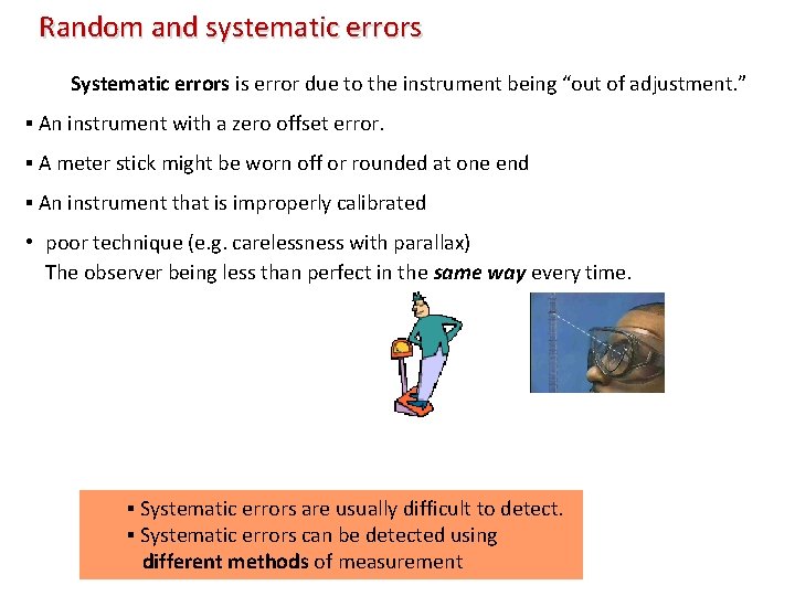
Random and systematic errors Systematic errors is error due to the instrument being “out of adjustment. ” ▪ An instrument with a zero offset error. ▪ A meter stick might be worn off or rounded at one end ▪ An instrument that is improperly calibrated • poor technique (e. g. carelessness with parallax) The observer being less than perfect in the same way every time. ▪ Systematic errors are usually difficult to detect. ▪ Systematic errors can be detected using different methods of measurement

RE SE precise, not accurate RE SE accurate, not precise RE SE neither precise, nor accurate RE SE both accurate and precise ▪ A measurement is said to be accurate if it has little systematic errors. ▪ A measurement is said to be precise if it has little random errors. ▪ A measurement can be of great precision but be inaccurate (for example, if the instrument used had a zero offset error).

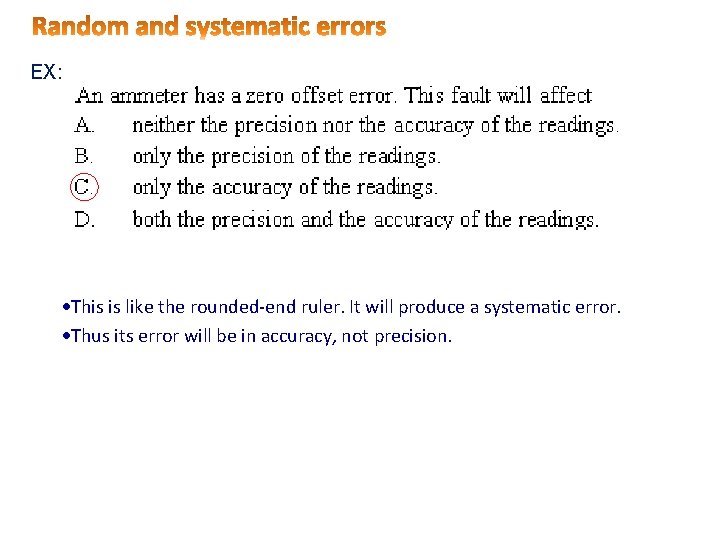
EX: This is like the rounded-end ruler. It will produce a systematic error. Thus its error will be in accuracy, not precision.

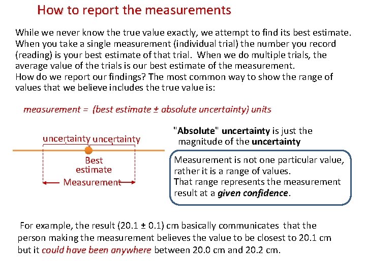
How to report the measurements While we never know the true value exactly, we attempt to find its best estimate. When you take a single measurement (individual trial) the number you record (reading) is your best estimate of that trial. When we do multiple trials, the average value of the trials is our best estimate of the measurement. How do we report our findings? The most common way to show the range of values that we believe includes the true value is: we believe measurement = (best estimate ± absolute uncertainty) units uncertainty Best estimate Measurement "Absolute" uncertainty is just the magnitude of the uncertainty Measurement is not one particular value, rather it is a range of values. That range represents the measurement result at a given confidence For example, the result (20. 1 ± 0. 1) cm basically communicates that the person making the measurement believes the value to be closest to 20. 1 cm but it could have been anywhere between 20. 0 cm and 20. 2 cm. anywhere

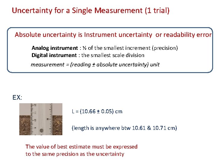
Uncertainty for a Single Measurement (1 trial) Absolute uncertainty is Instrument uncertainty or readability error Analog instrument : ½ of the smallest increment (precision) Digital instrument : the smallest scale division measurement = (reading ± absolute uncertainty) unit EX: L = (10. 66 ± 0. 05) cm (length is anywhere btw 10. 61 & 10. 71 cm) The value of best estimate must be expressed to the same precision as the uncertainty

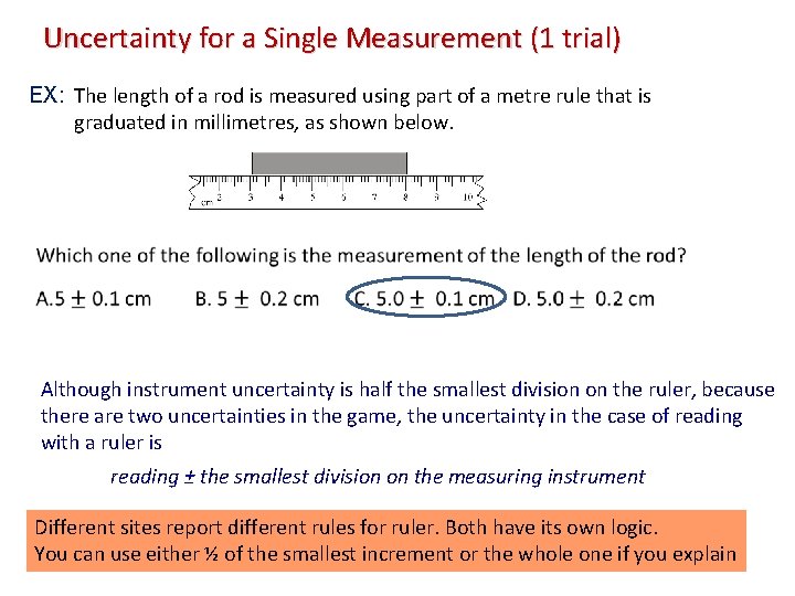
Uncertainty for a Single Measurement (1 trial) EX: The length of a rod is measured using part of a metre rule that is graduated in millimetres, as shown below. Although instrument uncertainty is half the smallest division on the ruler, because there are two uncertainties in the game, the uncertainty in the case of reading with a ruler is reading ± the smallest division on the measuring instrument Different sites report different rules for ruler. Both have its own logic. You can use either ½ of the smallest increment or the whole one if you explain

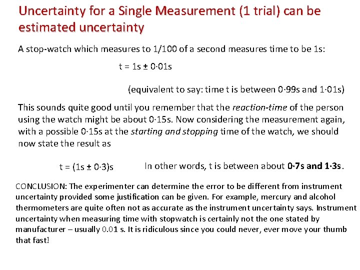
Uncertainty for a Single Measurement (1 trial) can be estimated uncertainty A stop-watch which measures to 1/100 of a second measures time to be 1 s: t = 1 s ± 0· 01 s (equivalent to say: time t is between 0· 99 s and 1· 01 s) This sounds quite good until you remember that the reaction-time of the person using the watch might be about 0· 15 s. Now considering the measurement again, with a possible 0· 15 s at the starting and stopping time of the watch, we should now state the result as t = (1 s ± 0· 3)s In other words, t is between about 0· 7 s and 1· 3 s. CONCLUSION: The experimenter can determine the error to be different from instrument uncertainty provided some justification can be given. For example, mercury and alcohol provided some justification thermometers are quite often not as accurate as the instrument uncertainty says. Instrument uncertainty when measuring time with stopwatch is certainly not the one stated by manufacturer – usually 0. 01 s. It is ridiculous since you could never, ever move your thumb that fast!

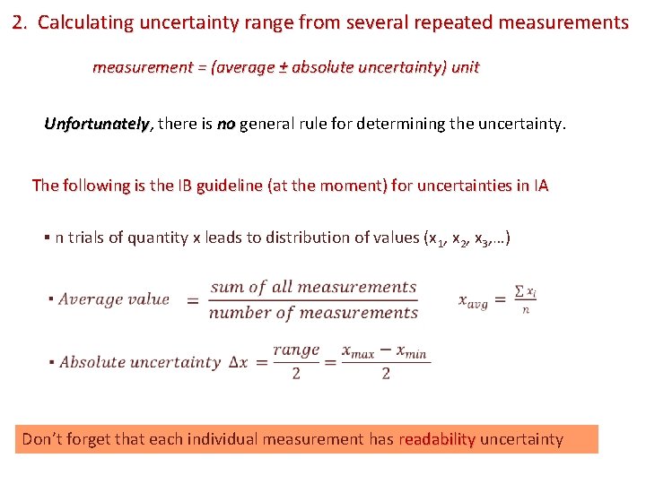
2. Calculating uncertainty range from several repeated measurements measurement = (average ± absolute uncertainty) unit Unfortunately, there is no general rule for determining the uncertainty. Unfortunately The following is the IB guideline (at the moment) for uncertainties in IA ▪ n trials of quantity x leads to distribution of values (x 1, x 2, x 3, …) Don’t forget that each individual measurement has readability uncertainty eadability

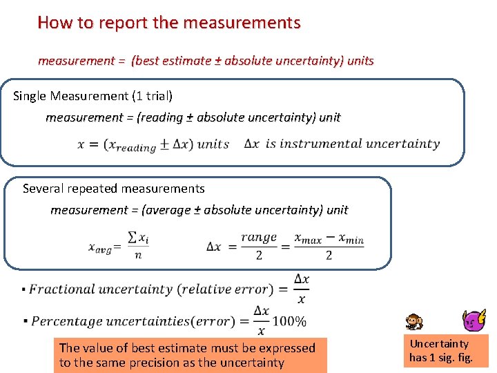
How to report the measurements measurement = (best estimate ± absolute uncertainty) units Single Measurement (1 trial) measurement = (reading ± absolute uncertainty) unit Several repeated measurements measurement = (average ± absolute uncertainty) unit The value of best estimate must be expressed to the same precision as the uncertainty Uncertainty has 1 sig. fig.

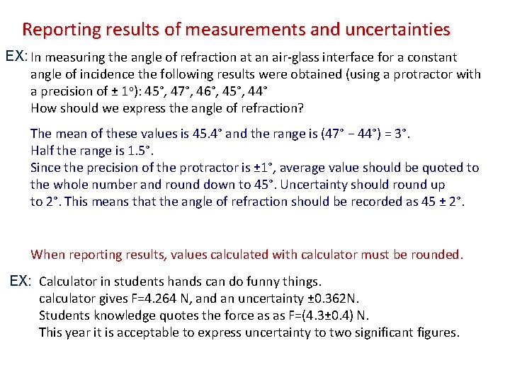
Reporting results of measurements and uncertainties EX: In measuring the angle of refraction at an air-glass interface for a constant angle of incidence the following results were obtained (using a protractor with a precision of ± 1 o): 45°, 47°, 46°, 45°, 44° How should we express the angle of refraction? The mean of these values is 45. 4° and the range is (47° − 44°) = 3°. Half the range is 1. 5°. Since the precision of the protractor is ± 1°, average value should be quoted to the whole number and round down to 45°. Uncertainty should round up to 2°. This means that the angle of refraction should be recorded as 45 ± 2°. When reporting results, values calculated with calculator must be rounded. EX: Calculator in students hands can do funny things. calculator gives F=4. 264 N, and an uncertainty ± 0. 362 N. Students knowledge quotes the force as as F=(4. 3± 0. 4) N. This year it is acceptable to express uncertainty to two significant figures.

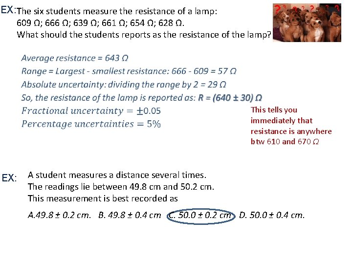
EX: The six students measure the resistance of a lamp: 609 Ω; 666 Ω; 639 Ω; 661 Ω; 654 Ω; 628 Ω. What should the students reports as the resistance of the lamp? This tells you immediately that resistance is anywhere btw 610 and 670 Ω EX: A student measures a distance several times. The readings lie between 49. 8 cm and 50. 2 cm. This measurement is best recorded as A. 49. 8 ± 0. 2 cm. B. 49. 8 ± 0. 4 cm C. 50. 0 ± 0. 2 cm D. 50. 0 ± 0. 4 cm.

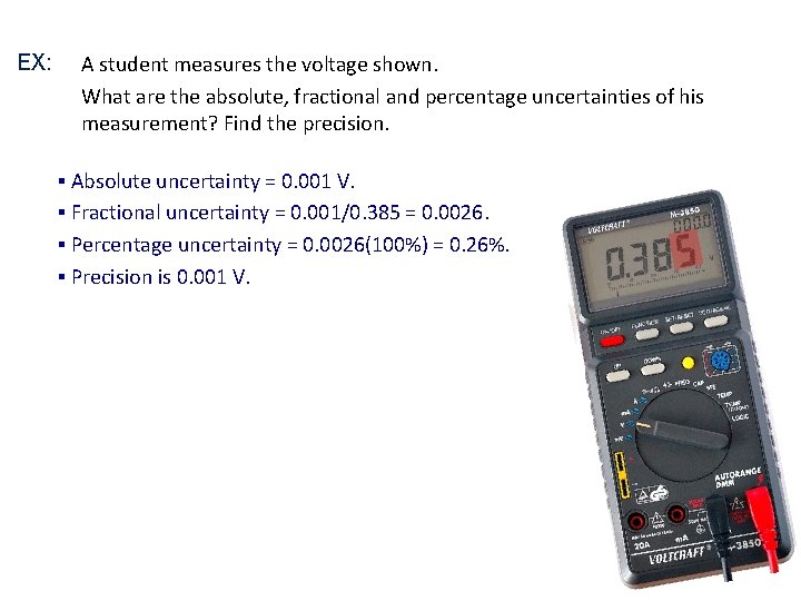
EX: A student measures the voltage shown. What are the absolute, fractional and percentage uncertainties of his measurement? Find the precision. ▪ Absolute uncertainty = 0. 001 V. ▪ Fractional uncertainty = 0. 001/0. 385 = 0. 0026. ▪ Percentage uncertainty = 0. 0026(100%) = 0. 26%. ▪ Precision is 0. 001 V.

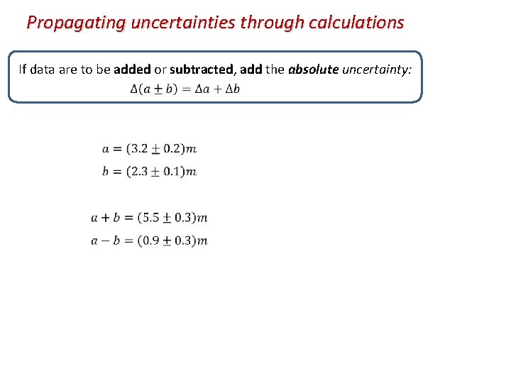
Propagating uncertainties through calculations If data are to be added or subtracted, add the absolute uncertainty:

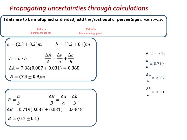
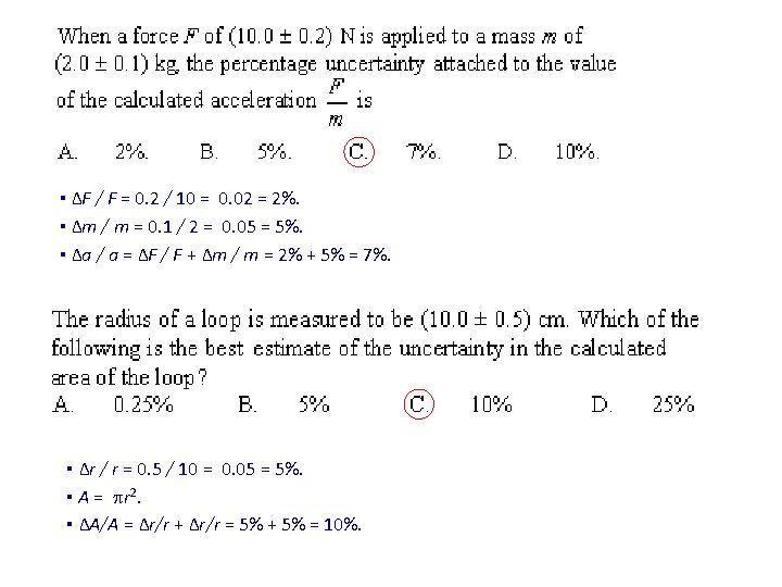
Propagating uncertainties through calculations If data are to be multiplied or divided, add the fractional or percentage uncertainty:

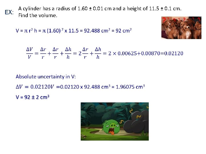
A cylinder has a radius of 1. 60 ± 0. 01 cm and a height of 11. 5 ± 0. 1 cm. EX: Find the volume.

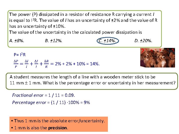
The power (P) dissipated in a resistor of resistance R carrying a current I is equal to I 2 R. The value of I has an uncertainty of ± 2% and the value of R has an uncertainty of ± 10%. The value of the uncertainty in the calculated power dissipation is A. ± 8%. B. ± 12%. C. ± 14%. D. ± 20%. A student measures the length of a line with a wooden meter stick to be 11 mm 1 mm. What is the percentage error or uncertainty in her measurement? Fractional error = 1 / 11 = 0. 09. Percentage error = (1 / 11) · 100% = 9% ▪ Thus 1 mm is the absolute error/uncertainty. ▪ 1 mm is also the precision.

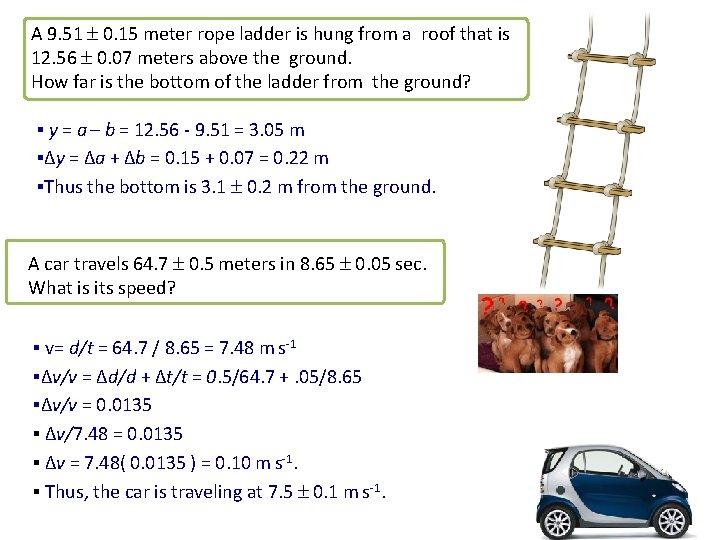
A 9. 51 0. 15 meter rope ladder is hung from a roof that is 12. 56 0. 07 meters above the ground. How far is the bottom of the ladder from the ground? ▪ y = a – b = 12. 56 - 9. 51 = 3. 05 m ▪∆y = ∆a + ∆b = 0. 15 + 0. 07 = 0. 22 m ▪Thus the bottom is 3. 1 0. 2 m from the ground. A car travels 64. 7 0. 5 meters in 8. 65 0. 05 sec. What is its speed? ▪ v= d/t = 64. 7 / 8. 65 = 7. 48 m s-1 ▪∆v/v = ∆d/d + ∆t/t = 0. 5/64. 7 +. 05/8. 65 ▪∆v/v = 0. 0135 ▪ ∆v/7. 48 = 0. 0135 ▪ ∆v = 7. 48( 0. 0135 ) = 0. 10 m s-1. ▪ Thus, the car is traveling at 7. 5 0. 1 m s-1.

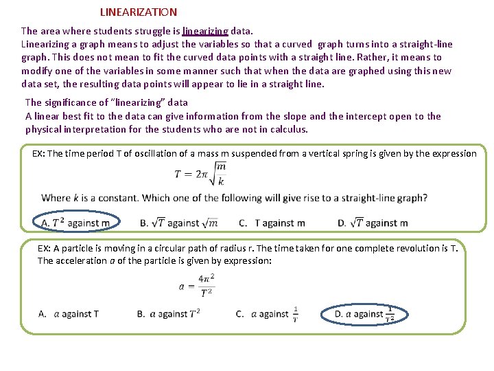
LINEARIZATION The area where students struggle is linearizing data. Linearizing a graph means to adjust the variables so that a curved graph turns into a straight-line graph. This does not mean to fit the curved data points with a straight line. Rather, it means to modify one of the variables in some manner such that when the data are graphed using this new data set, the resulting data points will appear to lie in a straight line. The significance of “linearizing” data A linear best fit to the data can give information from the slope and the intercept open to the physical interpretation for the students who are not in calculus. EX: The time period T of oscillation of a mass m suspended from a vertical spring is given by the expression EX: A particle is moving in a circular path of radius r. The time taken for one complete revolution is T. The acceleration a of the particle is given by expression:

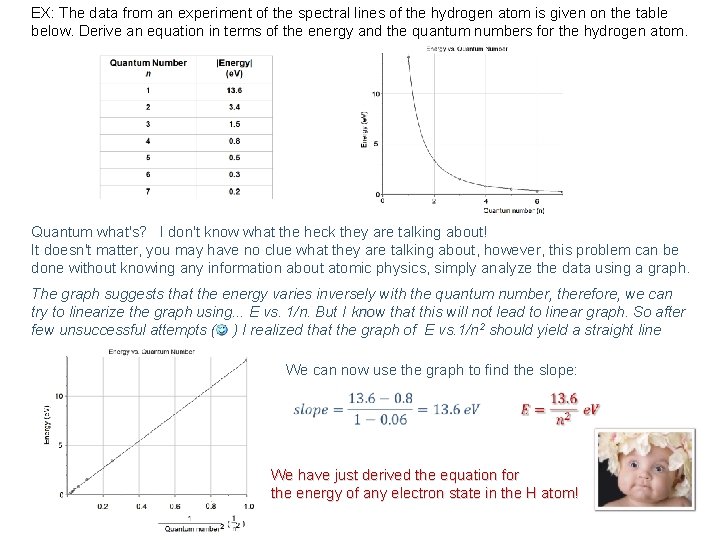
EX: The data from an experiment of the spectral lines of the hydrogen atom is given on the table below. Derive an equation in terms of the energy and the quantum numbers for the hydrogen atom. Quantum what's? I don't know what the heck they are talking about! It doesn't matter, you may have no clue what they are talking about, however, this problem can be done without knowing any information about atomic physics, simply analyze the data using a graph. The graph suggests that the energy varies inversely with the quantum number, therefore, we can try to linearize the graph using. . . E vs. 1/n. But I know that this will not lead to linear graph. So after few unsuccessful attempts ( ) I realized that the graph of E vs. 1/n 2 should yield a straight line We can now use the graph to find the slope: We have just derived the equation for the energy of any electron state in the H atom!

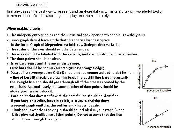
DRAWING A GRAPH In many cases, the best way to present and analyze data is to make a graph. A wonderful tool of communication. Graphs also let you display uncertainties nicely. When making graphs: 1. The independent variable is on the x-axis and the dependent variable is on the y-axis. 2. Every graph should have a title that this concise but descriptive, in the form ‘Graph of (dependent variable) vs. (independent variable)’. 3. The scales of the axes should suit the data ranges. 4. The axes should be labeled with the variable, units, and instrument uncertainties. 5. The data points should be clear. 7. Error bars represent the uncertainty range. Error bars should be shown correctly (using a straight-edge). 8. Data points (average value ONLY!) should not be connected dot-to-dot fashion. A line of best fit should be drawn instead. The best fit line is not necessarily the straight line and should pass through all of the crosses created by the error bars. Approximately the same number of data points should be above your line as below it. 9. Each point that does not fit with the best fit line should be identified. If you have an outlier, leave it as it is, discuss it, and the draw a second graph omitting the outlier and discuss it again. 10. Think about whether the origin should be included in your graph (what is the physical significance of that point? ) Do not assume that the line should pass through the origin.

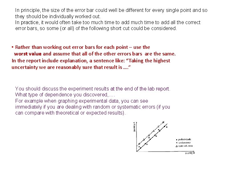
In principle, the size of the error bar could well be different for every single point and so they should be individually worked out. In practice, it would often take too much time to add all the correct In practice error bars, so some (or all) of the following short cut could be considered. ▪ Rather than working out error bars for each point – use the worst value and assume that all of the other errors bars are the same. In the report include explanation, a sentence like: “Taking the highest uncertainty we are reasonably sure that result is …. ” You should discuss the experiment results at the end of the lab report What type of dependence you discovered, …. For example when graphing experimental data, you can see immediately if you are dealing with random or systematic errors (if you can compare with theoretical or expected results).

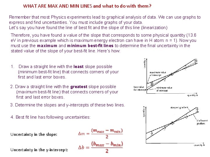
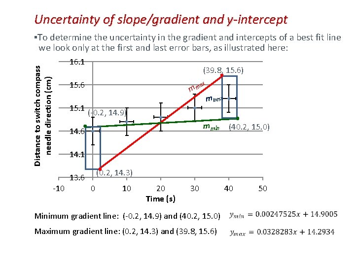
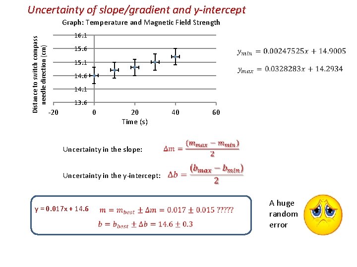
WHAT ARE MAX AND MIN LINES and what to do with them? Remember that most Physics experiments lead to graphical analysis of data. We can use graphs to express and find uncertainties. You must include graphs of your data. Let’s say you have found the line of best fit and the slope of this line (linearization) Therefore, you have found a value of the slope that corresponds to some physical quantity (13. 6 e. V in previous example which is maximum energy electron can have in H atom: n = 1). Now you must use the maximum and minimum best-fit lines to determine the final uncertainty in the stated value of the slope of your best-fit line. Here’s how: 1. Draw a straight line with the least slope possible (minimum best-fit line) that connects corners of your first and last error boxes. 2. Draw a straight line with the greatest slope possible (maximum best-fit line) that connects corners of your first and last error boxes. 3. Determine the slopes and y-intercepts of these two lines. 4. Best fit line has following uncertainties: Uncertainty in the slope: Uncertainty in the y-intercept:

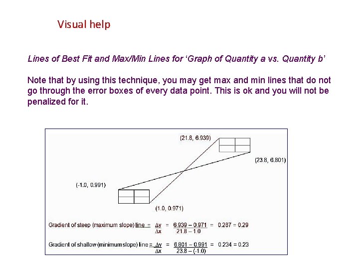
Visual help Lines of Best Fit and Max/Min Lines for ‘Graph of Quantity a vs. Quantity b’ Note that by using this technique, you may get max and min lines that do not go through the error boxes of every data point. This is ok and you will not be penalized for it.

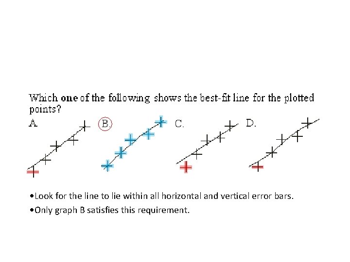
Look for the line to lie within all horizontal and vertical error bars. Only graph B satisfies this requirement.

IB has a requirement that when you conduct an experiment of your own design, you must have five variations in your independent variable. And for each variation of your independent variable you must conduct five trials to gather the values of the dependent variable. The five values for each dependent variable will then be averaged. Here is an example of perfect student’s work.

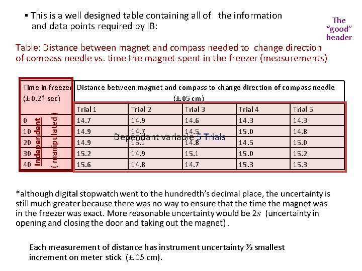
▪ This is a well designed table containing all of the information and data points required by IB: The “good” header Table: Distance between magnet and compass needed to change direction of compass needle vs. time the magnet spent in the freezer (measurements) ( manipulated ) Independent Time in freezer Distance between magnet and compass to change direction of compass needle (± 0. 2* sec) (±. 05 cm) Trial 1 Trial 2 Trial 3 Trial 4 Trial 5 0 14. 7 14. 9 14. 6 14. 3 10 14. 9 14. 7 14. 5 15. 0 14. 8 Dependant variable 5 Trials 20 14. 9 15. 1 14. 8 14. 5 15. 0 30 15. 2 14. 9 15. 1 15. 0 15. 2 40 15. 6 14. 8 14. 7 15. 3 Each measurement of distance has instrument uncertainty ½ smallest increment on meter stick (±. 05 cm).

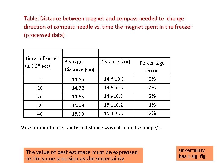
Table: Distance between magnet and compass needed to change direction of compass needle vs. time the magnet spent in the freezer (processed data) Time in freezer Average (± 0. 2* sec) Distance (cm) Percentage error 0 14. 56 14. 6 ± 0. 3 2% 10 14. 78 14. 8± 0. 3 2% 20 14. 86 14. 9± 0. 3 2% 30 15. 08 15. 1± 0. 2 1% 40 15. 30 15. 3± 0. 3 2% Measurement uncertainty in distance was calculated as range/2 The value of best estimate must be expressed to the same precision as the uncertainty Uncertainty has 1 sig. fig.

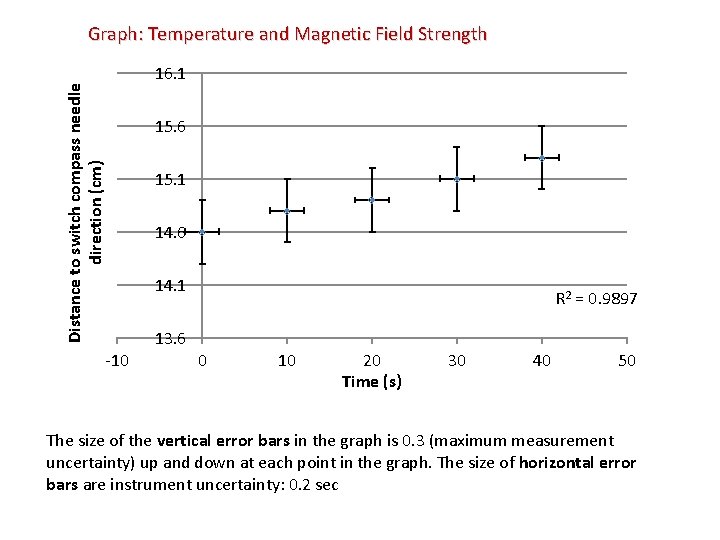
Distance to switch compass needle direction (cm) Graph: Temperature and Magnetic Field Strength -10 16. 1 15. 6 15. 1 14. 6 14. 1 13. 6 R 2 = 0. 9897 0 10 20 Time (s) 30 40 50 The size of the vertical error bars in the graph is 0. 3 (maximum measurement uncertainty) up and down at each point in the graph. The size of horizontal error bars are instrument uncertainty: 0. 2 sec

Uncertainty of slope/gradient and y-intercept Distance to switch compass needle direction (cm) ▪To determine the uncertainty in the gradient and intercepts of a best fit line we look only at the first and last error bars, as illustrated here: -10 16. 1 (39. 8, 15. 6) 15. 6 15. 1 ax mm m best (-0. 2, 14. 9) mmin 14. 6 (40. 2, 15. 0) 14. 1 13. 6 (0. 2, 14. 3) 0 10 20 Time (s) 30 40 Minimum gradient line: (-0. 2, 14. 9) and (40. 2, 15. 0) Maximum gradient line: (0. 2, 14. 3) and (39. 8, 15. 6) 50

Uncertainty of slope/gradient and y-intercept Distance to switch compass needle direction (cm) Graph: Temperature and Magnetic Field Strength 16. 1 15. 6 15. 1 14. 6 14. 1 13. 6 -20 0 20 Time (s) 40 60 Uncertainty in the slope: Uncertainty in the y-intercept: y = 0. 017 x + 14. 6 A huge random error