Decision Making under Uncertainty 1 Introduction n n

Decision Making under Uncertainty 1

Introduction n n In many decisions the consequences of the alternative courses of action cannot be predicted with certainty. A company which is considering the launch of a new product will be uncertain about how successful the product will be. 2

n An expected value can be regarded as an average outcome if a process is repeated a large number of times, this approach is arguably most relevant to situations where a decision is made repeatedly over a long period. 3

n n In many situations, however, the decision is not made repeatedly, and the decision maker may only have one opportunity to choose the best course of action. In these circumstances some people might prefer the least risky course of action. 4

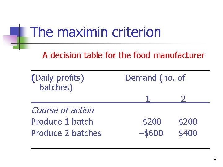
The maximin criterion A decision table for the food manufacturer (Daily profits) batches) Demand (no. of 1 2 Course of action Produce 1 batch Produce 2 batches $200 –$600 $400 5

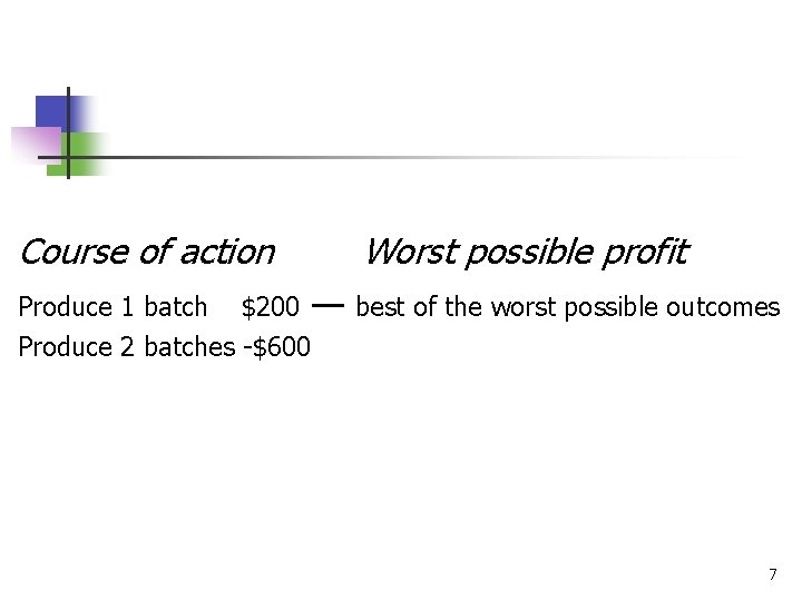
n n Given these potential profits and losses, how should the manufacturer make his decision? According to the maximin criterion the manufacturer should first identify the worst possible outcome for each course of action and then choose the alternative yielding the best of these worst outcomes. 6

Course of action Worst possible profit Produce 1 batch $200 — best of the worst possible outcomes Produce 2 batches -$600 7

n n n minimax for cost criterion The main problem with the maximin criterion is its inherent pessimism. Each option is assessed only on its worst possible outcome so that all other possible outcomes are ignored. 8

n The extreme risk aversion which is implied by the maximin criterion may be appropriate where decisions involve public safety or possible irreversible damage to the environment. 9

The expected monetary value (EMV) criterion n n An expected value can be regarded as an average result which is obtained if a process is repeated a large number of times. This may make the criterion particularly appropriate for the retailer who will be repeating his decision day after day. 10

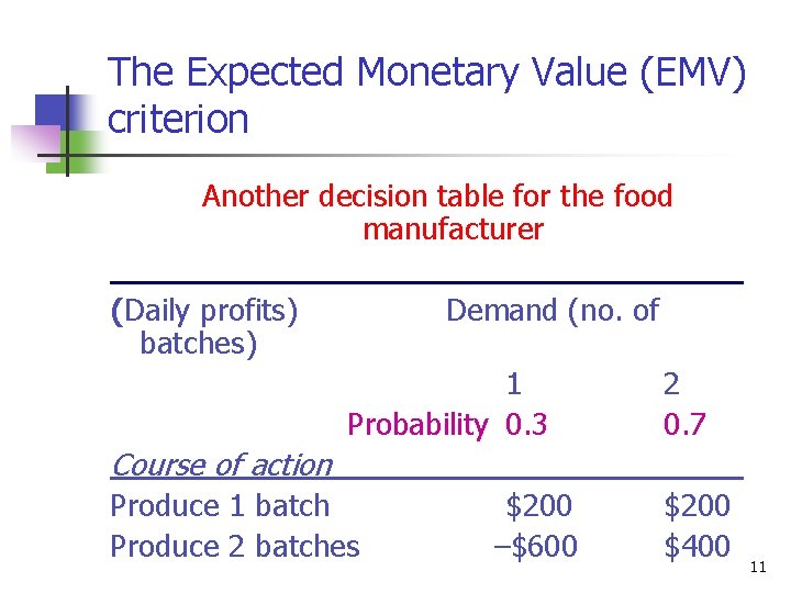
The Expected Monetary Value (EMV) criterion Another decision table for the food manufacturer (Daily profits) batches) Demand (no. of 1 Probability 0. 3 2 0. 7 Course of action Produce 1 batch Produce 2 batches $200 –$600 $200 $400 11

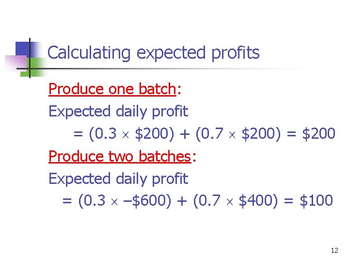
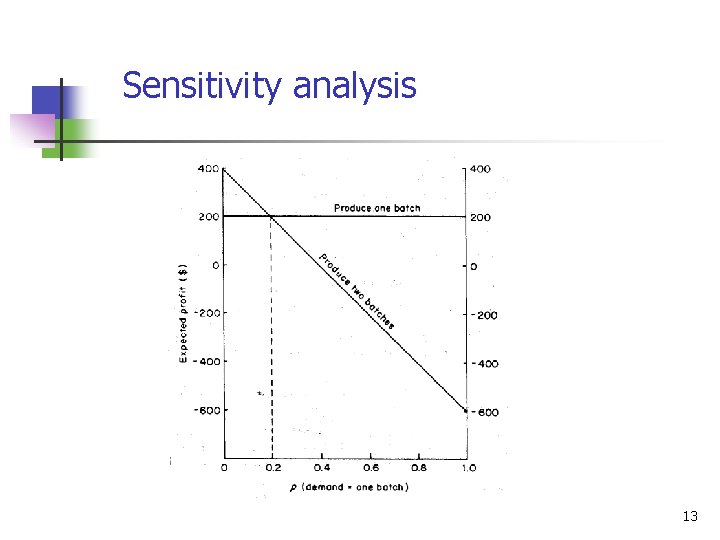
Calculating expected profits Produce one batch: Expected daily profit = (0. 3 $200) + (0. 7 $200) = $200 Produce two batches: Expected daily profit = (0. 3 –$600) + (0. 7 $400) = $100 12

Sensitivity analysis 13

Limitations of the EMV criterion n It assumes that the decision maker is neutral to risk It assumes a linear value function for money It considers only one attribute - money 14

n n n n Refer to Table 5. 3 The expected returns for design 1: 2. 3 m The expected returns for design 2: 4. 3 m Design 2 should be selected based on EMV would this really be your preferred course of action? this is a one-off decision, and there is therefore no chance of recouping losses on subsequent repetitions of the decision. The EMV criterion therefore fails to take into account the attitude to risk of the decision maker. 15

Single-attribute utility n n The attitude to risk of a decision maker can be assessed bv eliciting a utility function. The site selection problem is used To illustrate how a utility function can be derived. 16

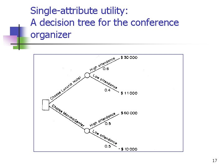
Single-attribute utility: A decision tree for the conference organizer 17

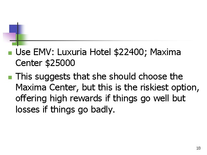
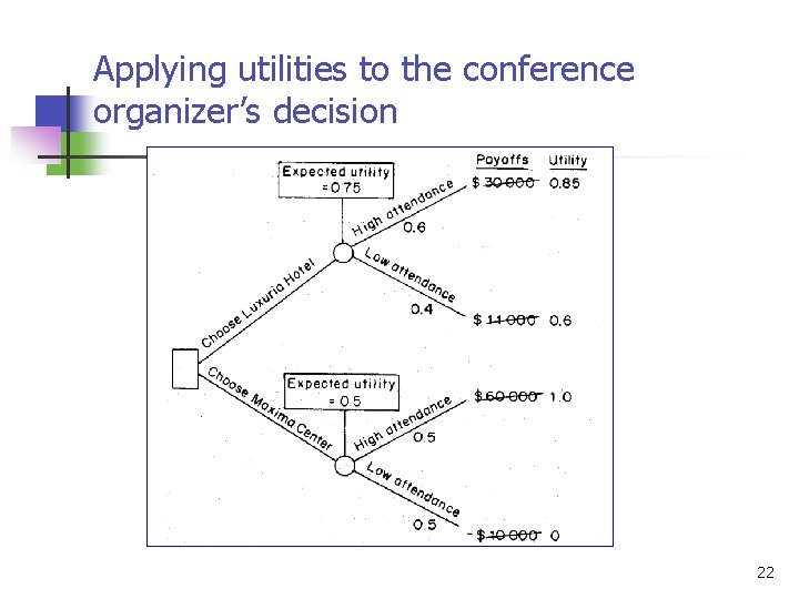
n n Use EMV: Luxuria Hotel $22400; Maxima Center $25000 This suggests that she should choose the Maxima Center, but this is the riskiest option, offering high rewards if things go well but losses if things go badly. 18

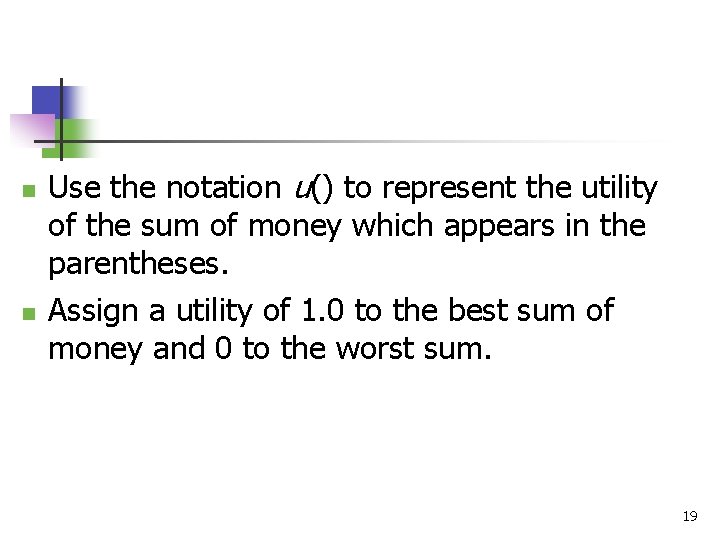
n n Use the notation u() to represent the utility of the sum of money which appears in the parentheses. Assign a utility of 1. 0 to the best sum of money and 0 to the worst sum. 19

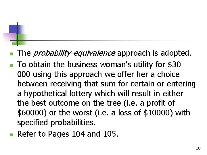
n n n The probability-equivalence approach is adopted. To obtain the business woman's utility for $30 000 using this approach we offer her a choice between receiving that sum for certain or entering a hypothetical lottery which will result in either the best outcome on the tree (i. e. a profit of $60000) or the worst (i. e. a loss of $10000) with specified probabilities. Refer to Pages 104 and 105. 20

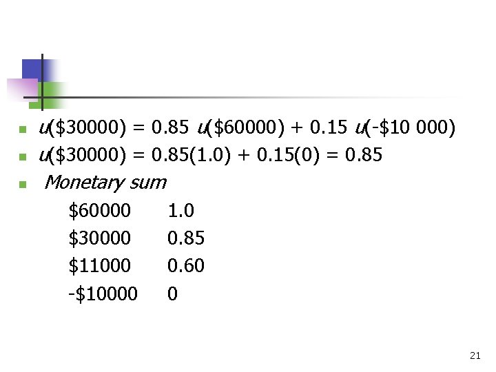
n n n u($30000) = 0. 85 u($60000) + 0. 15 u(-$10 000) u($30000) = 0. 85(1. 0) + 0. 15(0) = 0. 85 Monetary sum $60000 $30000 $11000 -$10000 1. 0 0. 85 0. 60 0 21

Applying utilities to the conference organizer’s decision 22

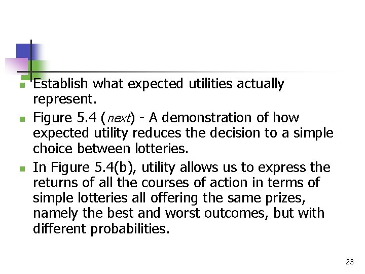
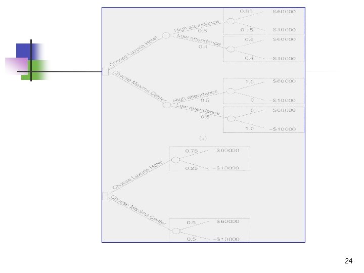
n n n Establish what expected utilities actually represent. Figure 5. 4 (next) - A demonstration of how expected utility reduces the decision to a simple choice between lotteries. In Figure 5. 4(b), utility allows us to express the returns of all the courses of action in terms of simple lotteries all offering the same prizes, namely the best and worst outcomes, but with different probabilities. 23

24

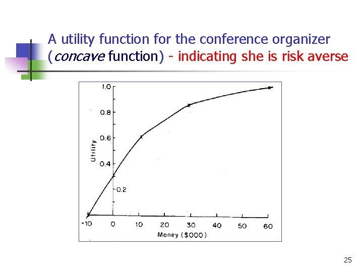
A utility function for the conference organizer (concave function) - indicating she is risk averse 25

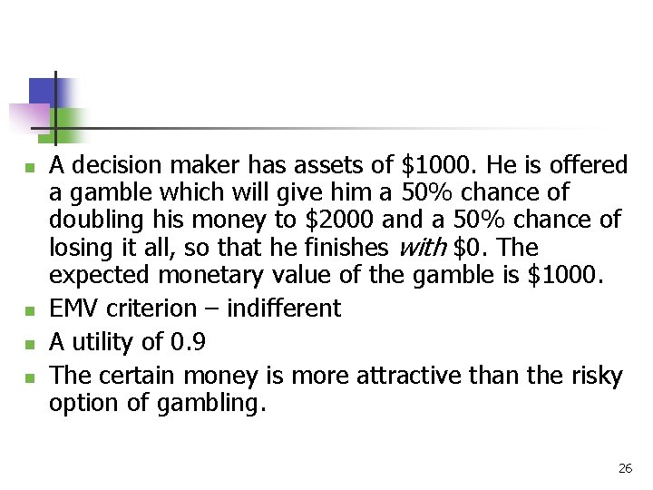
n n A decision maker has assets of $1000. He is offered a gamble which will give him a 50% chance of doubling his money to $2000 and a 50% chance of losing it all, so that he finishes with $0. The expected monetary value of the gamble is $1000. EMV criterion – indifferent A utility of 0. 9 The certain money is more attractive than the risky option of gambling. 26

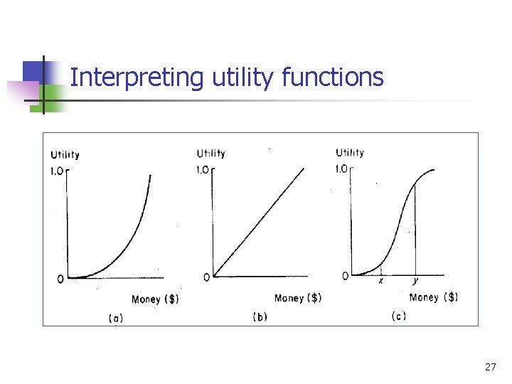
Interpreting utility functions 27

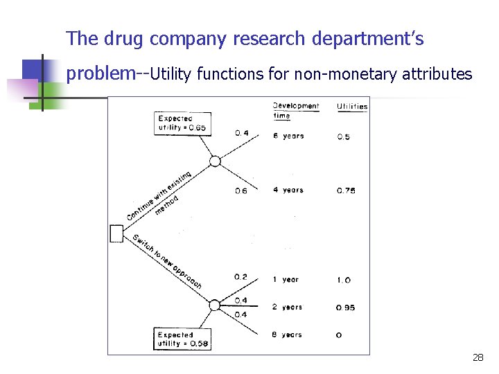
The drug company research department’s problem--Utility functions for non-monetary attributes 28

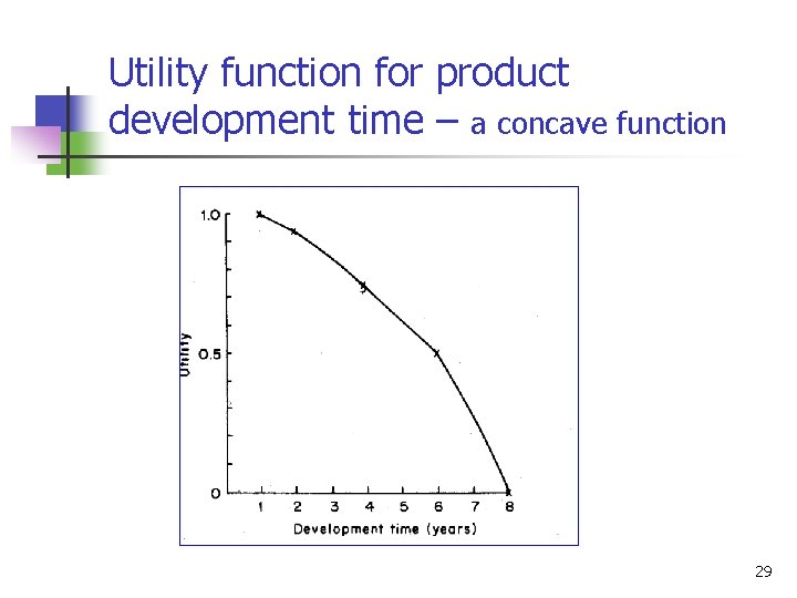
Utility function for product development time – a concave function 29

The axioms of utility n n Axiom 1: The complete ordering axiom To satisfy this axiom the decision maker must be able to place all lotteries in order of preference. 30

n n Axiom 2: The transitivity axiom If the decision maker prefers lottery A to lottery B and lottery B to lottery C then, if he conforms to this axiom, he must also prefer lottery A to lottery C. 31

n n Axiom 3: The continuity axiom states that there must be some value of p at which the decision maker will be indifferent between the two lotteries. (Figure 10) 32

n n Axiom 4: The substitution axiom if reward X appears as a reward in another lottery it can always be substituted by lottery 2 because the decision maker regards X and lottery 2 as being equally preferable. (Figure 11, 12) 33

n Axiom 5: Unequal probability axiom (Figure 5. 13) n Suppose that a decision maker prefers reward A to reward B. Then, according to this axiom, if he is offered two lotteries which only offer rewards A and B as possible outcomes he will prefer the lottery offering the highest probability of reward A. 34

n n Axiom 6: Compound lottery axiom (Figure 5. 14) If this axiom applies then a decision maker will be indifferent between a compound lottery and a simple lottery which offers the same rewards with the same probabilities. 35

n If the decision maker accepts the above six axioms then a utility function exists which represents his preferences. 36

More on utility elicitation n A disadvantage of probability-equivalence approach is that the decision maker may have difficulty in thinking in terms of probabilities like 0. 90 or 0. 95. The certainty-equivalence approach, which, in its most common form, only requires the decision maker to think in terms of 50: 50 gambles. Refer to Pages 116 and 117. 37

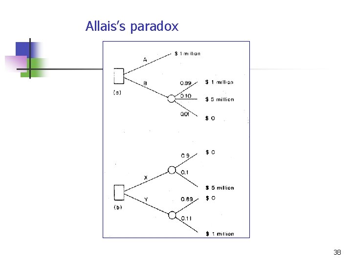
Allais’s paradox 38

n n n if you did choose options A and X your judgments are in conflict with utility theory. If we let u($5 m) = 1 and u($0) = 0, then selecting option A suggests that: u($1 m) is greater than 0. 89 u($1 m) + 0. 1 u($5 m) + 0. 01 u($0 m) i. e. u($1 m) exceeds 0. 89 u($1 m) + 0. 1 which implies: u($1 m) exceeds 0. 1/0. 11 39

n However, choosing X implies that: 0. 9 u($0) + 0. 1 u($5 m) exceeds 0. 89 u($0) + 0. 11 u($1 m) i. e. 0. 1 exceeds 0. 11 u($1 m) so that: u($1 m) is less than 0. 1/0. 11 40

Multi-attribute utility n n n Involve uncertainty and multiple attributes The 'divide and conquer' philosophy applies. By dividing the problem into small parts and allowing the decision maker to focus on each small part separately we aim to simplify his judgmental task. 41

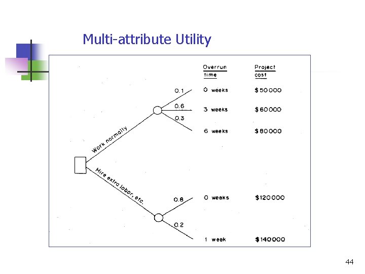
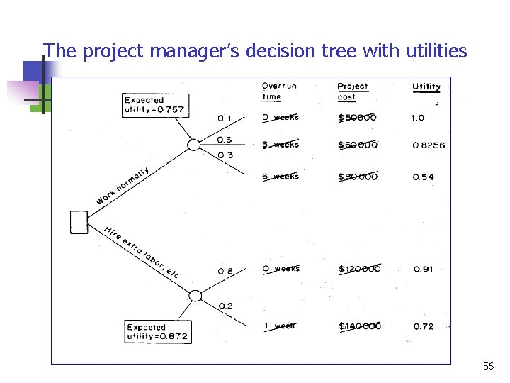
n n n To illustrate the approach let us consider the following problem which involves just two attributes. The overhaul is asked to be finished in 12 weeks. The company has two conflicting objectives: (1) minimize the time that the project overruns the target date and (2) minimize the cost of the project. 42

n n The project manager has two options: (1) work normally or (2) hire extra labor and work 24 -hour shifts. This process of deriving a multi-attribute utility function is simplified if certain assumptions can be made. The most important of these is that of mutual utility independence. 43

Multi-attribute Utility 44

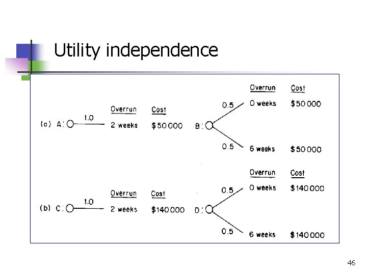
Utility independence Attribute A is utility independent of attribute B, if the decision maker’s preferences for gambles involving different levels of A, but the same level of B, do not depend on the level of attribute B. 45

Utility independence 46

n If project cost is also utility independent of overrun time (this will not automatically be the case) then we can say that overrun time and project cost are mutually utility independent. 47

n The great advantage of mutual utility independence, if it exists, is that it enables the decision maker to concentrate initially on deriving utility function for one attribute at a time without the need to worry about the other attributes. 48

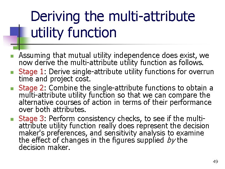
Deriving the multi-attribute utility function n n Assuming that mutual utility independence does exist, we now derive the multi-attribute utility function as follows. Stage 1: Derive single-attribute utility functions for overrun time and project cost. Stage 2: Combine the single-attribute functions to obtain a multi-attribute utility function so that we can compare the alternative courses of action in terms of their performance over both attributes. Stage 3: Perform consistency checks, to see if the multiattribute utility function really does represent the decision maker's preferences, and sensitivity analysis to examine the effect of changes in the figures supplied by the decision maker. 49

Deriving the multi-attribute utility function n n Assuming that mutual utility independence does exist, we now derive the multi-attribute utility function as follows. Stage 1: Derive single-attribute utility functions for overrun time and project cost. Stage 2: Combine the single-attribute functions to obtain a multi-attribute utility function so that we can compare the alternative courses of action in terms of their performance over both attributes. Stage 3: Perform consistency checks, to see if the multiattribute utility function really does represent the decision maker's preferences, and sensitivity analysis to examine the effect of changes in the figures supplied by the decision maker. 50

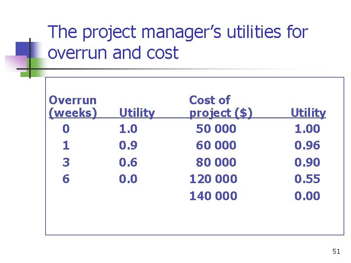
The project manager’s utilities for overrun and cost Overrun (weeks) 0 1 3 6 Utility 1. 0 0. 9 0. 6 0. 0 Cost of project ($) 50 000 60 000 80 000 120 000 140 000 Utility 1. 00 0. 96 0. 90 0. 55 0. 00 51

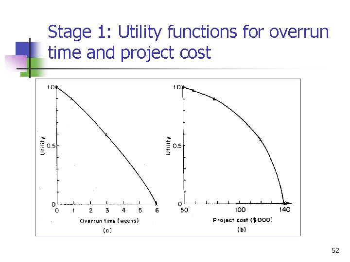
Stage 1: Utility functions for overrun time and project cost 52

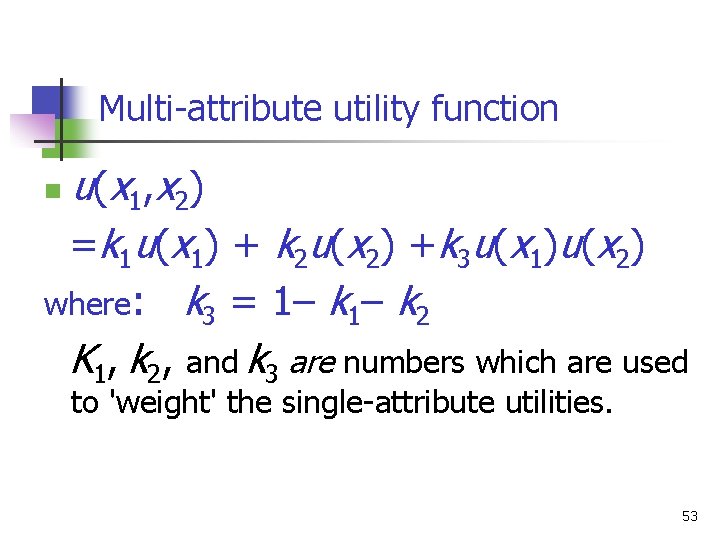
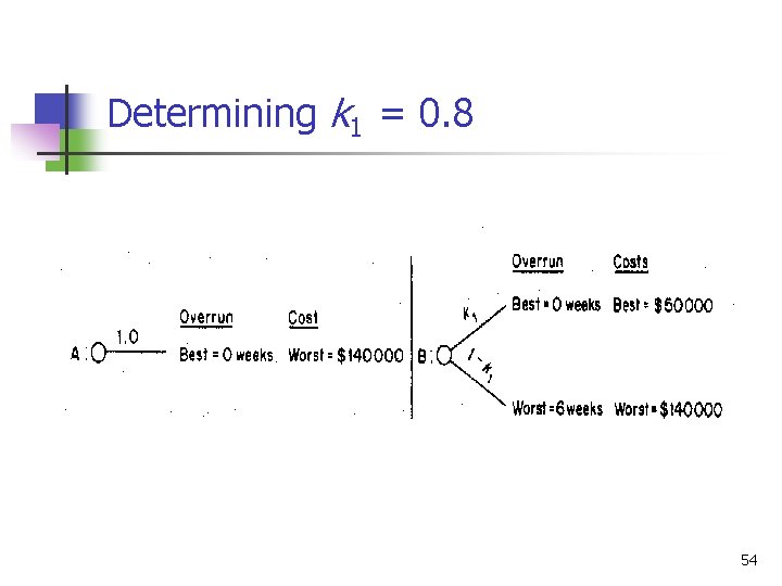
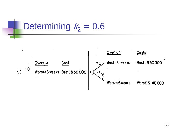
Multi-attribute utility function u ( x 1 , x 2 ) =k 1 u(x 1) + k 2 u(x 2) +k 3 u(x 1)u(x 2) where: k 3 = 1– k 2 K 1, k 2, and k 3 are numbers which are used n to 'weight' the single-attribute utilities. 53

Determining k 1 = 0. 8 54

Determining k 2 = 0. 6 55

The project manager’s decision tree with utilities 56