Decision making under uncertainty Uncertainty arise from Incomplete

Decision making under uncertainty Uncertainty arise from Incomplete Incorrectness of knowledge Decision theory = probability theory + utility theory Rational agents: select the action that maximizes the expected utility

Design of decision-theoretic agents Function DT-Agent(percept) returns an action static a set of probabilistic beliefs about the state of the world calculate updated probabilities for current state based on available evidence including current percept and previous actions calculate outcome probabilities for actions given action descriptions and probabilities of current state select action with highest expected utility given probabilities of outcomes and utility information Return action

Outline Ø Probability theory Bayesian Belief network Decision Theoretic Reasoning

Basic probability notions Prior probability (unconditional probability) Conditional probability P(A|B)= P(A B)/P(B) P(A B) =P(A|B)P(B)

Axioms of probability 0 P(A) 1 P(true)=1; P(false)=0 P(A B)=P(A)+P(B)-P(A B)

Bayes’ Rule P(Y|X)=P(X|Y)P(Y)/P(X) P(Y|X, E)=P(X|Y, E)P(Y|E)/P(X|E) Normalization P(M|S)=P(S|M)P(M)/[P(S|M)P(M)+ P(S| M)P( M)]

Conditional Independence X and Y are independent given Z P(X|Y, Z) = P(X|Z) P(Z|X, Y)= P(X, Y|Z)P(Z)= P(Z)P(X|Z)P(Y|Z)

Outline Probability theory Ø Bayesian Belief network Decision Theoretic Reasoning Sequential Decision theoretic reasoning

Belief Networks A DAG (directed acyclic graph) Each node is associated with a random variable Burglary Earthquake Alarm John. Calls Mary. Calls

Belief networks A set of random variables as nodes of the network A set of directed links or arrows connects pairs of nodes. “Direct influence” Each node has a conditional probability table that quantifies the effects that the parents have on nodes. The graph is a DAG

Conditional Probability Table Burglary Earthquake P(Alarm|Burglary, Earthquake) True false True 0. 95 0. 05 True False 0. 95 0. 05 False True 0. 29 0. 71 False 0. 001 0. 999

Bayesian Belief Network P(B). 001 P(E) Burglary Earthquake . 002 B E T T F F T F Alarm John. Calls Mary. Calls A T F P(J). 90. 05 A T F P(A). 95. 94. 29. 001 P(M) . 70. 10

Constructing Belief networks P(x 1, x 2, …, xn) = P(xn|xn-1, …, x 1)P(xn-1, …, x 1) = P(xn|xn-1, …, x 1) P(xn-1| xn-2, …, x 1)…P(x 2|x 1)P(x 1) P(Xi|Xi-1, …. , X 1)= inp(Xi|parente(Xi))

Representing joint probability distribution P(x 1, x 2, …, xn) = inp(xi|parente(xi)) P(J M A B E) = P(J|A)P(M|A)P(A| B E)P( B)P( E) = 0. 90*0. 70*0. 001*0. 999*0. 998 = 0. 00062

Conditional Independence relations in belief networks D-separation (direction-dependent separation): A set of nodes X is independent of another set Y given a set of evidence nodes Z. A set of nodes Z d-separates two set of nodes X and Y if every undirected path from a node X to a node Y is blocked given Z.

Path blocked conditions A path is blocked given a set of nodes E if there is a node Z for which one of the following conditions holds: 1. Z is in E and Z has one arrow on the path leading in and one arrow out 2. Z is in E and Z has both path arrows leading out 3. Neither Z nor any descendent of Z is in E, and both path arrows lead in to Z.

D-separation (2) (3) Z (1) X X Z Z E Y

independence of its nondescendents Um U 1 Z 1 j Znj X Y 1 Yn

Markov blanket and Conditional independence Um U 1 Z 1 j Znj X Y 1 Yn

A belief network for Car domain Battery Gas Radio Ignition Starts Moves

Examples of d-separation 1. Given Spark Plugs fire, Gas in the car and Car Radio plays are independent 2. Given Battery works, Gas and Radio are independent 3. Given no evidence at all, Gas and Radio are independent, but they becomes dependent given evidence about car Starts

Inference in belief network Diagnostic Intercausal Q E mixed E Q (Explain away) E Q Diagnostic causal E mixed

Singly connected Belief networks Singly connected network(Polytree): any two nodes can be connected by at most one undirected path

Causal support and Evidential Support Causal support EX+: evidence above X Evidential support EX-: evidence blow X EUiX: evidence connected to node Ui except X E+YiX: evidence connected to node Yi through its parents except for X

Compute P(X|E) in terms of EX+ and EX Compute EX+ by computing its effect on the parents of X and then passing the effect on X Compute EX- by computing its effect on the children of X and then passing the effect on to X

E X+ U 1 Um X Z 1 j Znj Y 1 Yn E X-

Calculation of P(X|E) in Singly connected belief network P(X|E) = P(X| EX-, EX+) = P(EX-|X, EX+)P(X| EX+)/ P(EX-|EX+) Due to X d-separates EX- and EX+, EX- and EX+ are independent = P(EX-|X)P(X| EX+)

P(X|E+) P(X|EX+)= u. P(X|u, EX+)P(u|EX+) u is a vector of assignment of values to all X’s parents Ui U d-separates X from EX+, P(X| EX+)= u. P(X|u) i. P(ui|EX+) = u. P(X|u) i. P(ui|EUiX)

P(EX-|X)= i. P(EyiX|X) = i yi zi. P(EyiX|X, yi, zi)P(yi, zi|X) = i yi zi. P(Eyi-|X, yi, zi)P(EyiX+|X, yi, zi) P(yi, zi|X) [Eyi- is independent of X and zi given yi EyiX+ is independent of X, yi, given zi ] = i yi P(Eyi-|yi) zi. P(EyiX+|zi) P(yi, zi|X)

Apply Bayes’s rule: P(zi |EyiX+)P(EyiX+) = i yi P(Eyi-|yi) zi P(zi) P(yi, zi|X) P(zi |EyiX+)P(EyiX+) = i yi P(Eyi-|yi) zi P(zi) P(yi|zi, X)P(zi|X) Z and X is d-separated, so P(zi)= P(zi|X) canceled out = i yi P(Eyi-|yi) zi i. P(zi |EyiX+) P(yi|zi, X)

The parents of Yi (Zij) are independent of each other = i yi P(Eyi-|yi) zi P(yi|zi, X) j. P(zij |EZijYi)

Belief Net Ask function Belief-Net-Ask(X) return a probability distribution over the values of x inputs X, a random variable SUPPORT-EXCEPT(X, null) function SUPPORT-EXCEPT if EVIDENCE? (X) then return observed point distribution for X else calculate P(E-XV|X)=EVIDENCE-EXCEPT(X, V) U PARENT[X] if U is empty then Return P(E-XV|X)P(X) else for each Ui in U calculate and store P(Ui|EUiX)=SUPPORT-EXCEPT(Ui, X) return P(E-XV|X) u. P(X|u) i. P(ui|EUiX)

function EVIDENCE-EXCEPT(X, V) returns P(E-XV|X) Y CHILDREN[X] –V if Y is empty then return a uniform distribution else for each Yi in Y do calculate P(E-Yi|yi) = EVIDENCE-EXCEPT(Yi, null) Zi PARENTS[Yi]-X for each Zij in Zi calculate P(Zij|E Zij Yi)=SUPPORT-EXCEPT(Zij, Yi) return i yi P(Eyi-|yi) zi P(yi|zi, X) j. P(zij |EZijYi)

Exact Inference in Bayesian networks Query variables, X Evidence variables, e, set of e: E Hidden variables, Y , non-evidence variables X= {X}U E U Y Typical query is the posterior probability P(X|e)

Burglary example Earthquake may cause alarm Burglary may cause alarm Alarm may cause Mary call Alarm may cause john call E B A J M

Inference by enumeration P(X|e) = αP(X, e) = α ∑y P(X, e, y) Take Burglary example, P(B|j, m)= α P(B, j, m) = α ∑e ∑a P(B, e, a, j, m) = α ∑e ∑a P(b)P(e)P(a|b, e)P(j|a)P(m|a) the complexity is O(n 2 n) = α P(b) ∑e P(e)∑a P(a|b, e)P(j|a)P(m|a)

P(b|j, m) = α x 0. 00059224 P(⌐b|j, m) = α x 0. 0014919 P(B|j, m) = α <0. 00059224, 0. 0014919> = <0. 284, 0. 716>

P(b)=. 001 P(e)=. 002 P(a|b, e)=0. 9 5 + + P(-e)=. 998 + P(-a|b, e)=0. 05 P(a|b, -e)=0. 94 P(j|a)=0. 90 P(j|-a)=0. 05 P(m|a)=0. 70 P(m|-a)=0. 01 P(-a|b, -e)=0. 06 P(j|a)=0. 90 P(j|-a)=0. 05 P(m|a)=0. 70 P(m|-a)=0. 01

Variable elimination algorithm P(B|j, m) = α P(b) ∑e P(e)∑a P(a|b, e)P(j|a)P(m|a) B E A J M These parts of expression with name of the associated variable are called factors

We store factor M, p(m|a) as a two-element vector f. M(A) = (p(m|a), p(m|-a)) Similarly for J The factor A is p(a|B, e) is a 2 x 2 x 2 matrix f. A(A, B, E) Factor sum out A as f. A’JM = ∑a f. A(a, B, E) × f. J(a) × f. M(a) = f. A(a, B, E) × f. J(a) × f. M(a) + f. A(-a, B, E) × f. J(-a) × f. M(-a). This is called pointwise product. Process E in the same way: sum out E from product f. E(E) and f. A’JM(B, E). f. E’A’JM(B) = f. E(e) × f. A’JM(B, e) + f. E(-e) × f. A’JM(B, -e) Finally we compute the answer by multiplying f. B(B) and f. E’A’JM(B). Namely P(B|j, m) = α f. B(B) × f. E’A’JM(B)

Pointwise product is not matrix multiplication. The trick is that any factor that does not depend on the variable to be summed out can be moved outside the summation process.

Variable elimination Suppose the query P(John. Calls |Burglary = true). P(J|b) = α P(b) ∑e. P(e) ∑a. P(a|b, e) P(J|a) ∑m. P(m|a) If we evaluate the expression from right to left, we note ∑m. P(m|a) = 1 by definition. Hence we don’t need to include it at the beginning. The variable M is irrelevant to this query. In general, we can remove any leaf node that is not a query variable or an evidence variable. Any variable that is not an ancestor of a query variable or evidence variable can be eliminated.

Multi-connected belief network Clustering methods Conditioning methods Stochastic simulation methods

Clustering methods Form Meganode: Springer+Rain C T F P(C)=. 5 P(S). 10. 50 Cloudy Rain Sprinkler S R P(W) T T F F T. 99 F. 90 T. 90 F. 00 Wet Grass C T F P(R). 80. 20

Clustering Cloudy Spr. +Rain S + RP(W) T T F F T. 99 F. 90 T. 90 F. 00 Wet Grass C TT TF FT FF T F . 08. 02. 72. 18. 40. 10

Cutset condtioning methods 0. 5 +Cloudy Sprinkler Rain Wet Grass -Cloudy Sprinkler -Cloudy Rain Wet Grass

Cutset Conditioning A set of variables that can be instantiated to yield polytrees is called a cutset Can set the accuracy of total probability up to certain likelihood, say, 0. 9

Stochastic simulation methods estimate P(X|E) We could sampling according to the prior probabilities and conditional probabilities For example, estimate P(Wet. Grass|Cloudy) Prior probability 0. 5 for cloudy or not cloudy and then conditional probabilities for Sprinkler and Rain…

Stochastic simulation The stochastic simulation might face the difficulty of getting accurate estimate probabilities for rare events, e. g. Sprinkler+rain, nuclear disaster The main difficulty of stochastically sampling method is that it takes long time to reach accurate probabilities of unlikely events A remedy is likelihood weighting method

Direct sampling methods SPS(x 1, x 2, …, xn)=∏i=1. . n. P(xi|parents(Xi)) Prior-Sample function PRIOR-SAMPLE(bn) returns an event sampled from the prior specified by bn inputs bn, a Bayesian network specifying joint distribution P(X 1, …, Xn) x ← an event with n elements for i=1 to n do xi ← a random sample from P(Xi|Parents(Xi)) return x

Example of direct sampling Sample order [Cloudy, Sprinkler, Rain, Wet. Grass] 1. Sample from P(Cloudy)=<0. 5, 0. 5> suppose this return true 2. Sample from P(Sprinkler|Coudy=true)=<0. 1, 0. 9> suppose this returns false 3. Sample from P(Rain|Cloudy=true)=<0. 8, 0. 2> ; suppose this returns true. 4. Sample from P(Wet. Grass|Sprinkler=false, Rain=true)=<0. 9, 0. 1>; suppose this return true. In this case, PRIOR-SAMPLE returns the event [true, false, true]

SPS(x 1, …. , xn) = Πi=1, n P(xi|parents(Xi)) Sampling depends on parent values. Lim N→∞ NPS(x 1, …xn)/N = SPS(x 1, …xn) = = P(x 1, …, xn)

Reject Sampling in Bayesian Networks function REJECTION-SAMPLING(X, e, bn, N) returns an estimate of P(X|e) Inputs: X, the query variable e, evidence specified as an event bn, a Bayesian network N, the total number of samples to be generated Local variables: N, a vector of counts over X, intially zero for j=1 to N do x ← PRIOR-SMAPLE(bn) if x is consistent with e then N[x] ← N[x]+1 where x is the value of X in x Return Normalize(N[X])

P’(X|e) = αNPS(X, e)=NPS(X, e)/NPS(e) The biggest problem with rejection sampling is that it rejects so many samples! estimate P(Rain|Red. Sky. At. Night=true)

Likelihood weighting avoids inefficient of rejecting sampling by generate only events that are consistent with the evidence e.

Function Likelihood-weighting(X, e, bn, N) returns an estimate of P(X|e) Inputs: X, the query variable e, evidence specified as an event bn, a Bayesian network N, the total number of samples to be generated local variables: W, a vector of weighted counts over X, initially zero for j=1 to N do x, w ←WEIGHTED-SAMPLE(bn, e) W[x] ←W[x]+w where x is the value of X in x Return Normalize(W[X])

function WEIGHTED-SAMPLE(bn, e) returns an event and a weight n x ← an event with n elements; w ← 1 for i=1 to n do If Xi has a value xi in e then w ← w x P(Xi=xi| parents(Xi)) else xi ← a random sample from return x, w P(Xi|parent(Xi))

1. Sample from P(Cloudy) =<0. 5, 0. 5> suppose return true 2. Sprinkler is an evidence variable with value true. Therefore, we set w ← w x P(Sprinkler=true|Cloudy=true)=0. 1. 3. Sample from P(Rain|Cloudy=true) = <0. 8, 0. 2>; suppose returns true. 4. Wet. Grass is an evidence variable with value true. Therefore, we set w ← w x P(Wet. Grass=true|Sprinkler=true, Rain=true) = 0. 099 Here WEIGHT-SAMPLE returns the event [true, true]

Because likelihood weighting uses all the samples generated, it can be much more efficient than rejection sampling. It will however, suffer a degradation in performance as the number of evidence variables increases. Because most samples will have very low weights and hence the weighted estimation will be dominated by the tiny fraction of samples that accord more than an infinitesimal likelihood to the evidence. The problem will exacerbated if the evidence variables occur late in the variable ordering.

algorithm for inference in BN. Query P(Rain|Sprinkler=true, Wet. Grass=true) Initial state [true, false, true] for [Cloudy, Sprinkler, Rain, Wet. Grass] at randomly Cloudy and Rain. 1. Cloudy is sampled, given the current values of its Markov blanket variables: in this case we sample from P(Cloudy|Sprinkler=true, Rain=false), Suppose the result is Cloudy= false. Then the new current state is [false, true, false, true] 2. Rain is sampled, given the current values of its Markov blanket variables; in this case, we sample from P(Rain|Cloudy=false, Sprinkler=true, Wet. Grass=true), Suppose this yields Rain=true. The new current state is [false, true, true].

function MCMC-Ask(X, e, bn, N) returns an estimate of P(X|e) local variables: N[X], a vector of count over X, initially zero Z, the nonevidence variables in bn x, the current state of the network, initially copied from e Initialize x with random values for variables in Z For j=1 to N do N[x]←N[x]+1 where x is the value of X in x for each Zi in Z do sample the value of Zi in x from P(Zi|mb(Zi)) given the values of MB(Zi) in x Return Normalize(N[X])

Why MCMC works? MCMC returns consistent estimate for posterior probabilities. The sampling process settles into a “dynamic equilibrium” in which the long-run fraction of time spent in each state is exactly proportional to its posterior probability. The property follows from the specific transition probability with which the process move from one state to another, as defined by the conditional distribution given the Markov blanket of the variables being sampled.

Let q(x→x’) be the probability that the process makes a transition from state x to state x’. This probability defines Markov chain on state space. Suppose we run the Markov chain for t steps and let πt(x) be the probability that the system is in state x at time t.

πt+1(x’)= ∑xπt(x) q(x→x’) We will say that the chain has reached its stationary distribution if πt+1 = πt Let us call this stationary distribution π, q(x→x’) for all x’ π(x’) = ∑xπ(x)

The property of detailed balance is that the expected “inflow” is equal to the expected “outflow” , namely: π(x) q(x→x’) = π(x’) q(x’→x) for all x, x’ ∑x π(x) q(x→x’) = ∑x π(x’) q(x’→x) = π(x’) ∑x q(x’→x) = π(x’)

Gibbs sampler Let Xi be the variable to be sampled and let Ẋi be all hidden variables other than Xi. Their values of current states are xi and ẋi. If we sample a new value xi’ for Xi conditionally on all the other variables, including the evidence, we have q(x→x’) = q((xi, ẋi ) →(xi’, ẋi ))= P(xi’| ẋi, e) The transition probability is called Gibbs sampler.

We show the Gibbs sampler is in detailed balance with the true posterior: π(x) q(x→x’) = P(x|e) P(xi’| ẋi, e) = P(xi, ẋi|e) P(xi’| ẋi, e) = P(xi|ẋi, e) P(xi’, ẋi|e) = q(x’→x) π(x’) = π(x’) q(x’→x)

Time and uncertainty Markov assumption: Current state depends on only finite history of previous states. First order Markov process: current state depends only on the previous state and not on earlier states.

1 st order and 2 nd order Markov processes Xt-2 Xt-1 Xt Xt Xt+1 Xt+2

Markov Assumption models P(Xt|X 0: t-1) = P(Xt|Xt-1) (transition model) P(Et|X 0: t, E 0: t-1) =P(Et|Xt) (sensor model) P(X 0) prior probability P(X 0, X 1, …. , Xt, E 1, E 2, …, Et) = P(X 0)∏i=1. . t P(Xi|Xi-1)P(Ei|Xi)

Bayesian network structure of umbrella world Transition model Rt-1 P(Rt) t f 0. 7 0. 3 Raint-1 Umbrellat-1 Raint+1 Rt P(Ut) T f 0. 9 0. 2 Umbrellat+1 Sensor model

Inference in Temporal Models Filtering and monitoring P(Xt|e 1: t) A process of computing distribution over cuurent state given evidence up to the present Prediction P(Xt+k|e 1: t) computing posterior distribution over the future state Smoothing or hindsight P(Xk|e 1: t): A process of computing distribution over past states given evidence up to the present Most likely explanation argmax x 1: t P(X 1: t|e 1: t) Given sequence of observation, find the sequence of states that is most likely to have generated the observations.

Filtering and Monitoring P(Xt|e 1: t) recursive estimation P(Xt+1|e 1: t+1) = f(et+1, P(Xt|e 1: t)) P(Xt+1|e 1: t+1) = P(Xt+1|e 1: t, et+1)) = α P(et+1| Xt+1, e 1: t)P(Xt+1|e 1: t) (Bayes’ rule) = α P(et+1| Xt+1)P(Xt+1|e 1: t) (Conditional independence)

X 0 X 1 Xk Xt E 1 Ek Et

P(Xt+1|e 1: t+1) = α P(et+1| Xt+1)P(Xt+1|e 1: t) = α P(et+1| Xt+1)Σxt. P(Xt+1|xt, e 1: t) P(xt|e 1: t ) = α P(et+1| Xt+1)Σxt. P(Xt+1|xt) P(xt|e 1: t ) (15. 3) Therefore, f 1: t+1 = αFORWARD(f 1: t , e 1: t )

Prediction P(Xt+k+1|e 1: t) =Σxt+k. P(Xt+k+1|xt+k) P(xt+k|e 1: t ) (15. 4)

Smoothing P(Xk|e 1: t) 1=<k<t P(Xk|e 1: t) = P(Xk|e 1: k, ek+1: t) =α P(Xk|e 1: k) P(ek+1: t | Xk, e 1: k) (Bayes’s rule) = α P(Xk|e 1: k) P(ek+1: t | Xk) = α f 1: kbk+1: t (15. 6) f 1: k = filtering forward from 1 to k bk+1: t = P(ek+1: t | Xk) =Σxk+1 P(ek+1: t | Xk, xk+1) P(xk+1|Xk) = Σxk+1 P(ek+1: t | xk+1) P(xk+1|Xk) =Σxk+1 P(ek+1, ek+2: t | xk+1) P(xk+1|Xk) =Σx P(e |x ) P(x |X ) (15. 7)

Finding the most likely sequence argmax x 1: t P(X 1: t|e 1: t) Suppose there is observation sequence of umbrella: [true, false, true] What is the most likely sequence of weathers to explain this? Viterbi algorithm: max x 1: t P(x 1: t, Xt+1|e 1: t+1) = α P(et+1| Xt+1) max xt (P(Xt+1|xt) max x 1: t-1 P(x 1, …, xt-1, xt|e 1: t)) (15. 9)

The equation 15. 9 is like filtering equation 15. 3 except 1. The forward message f 1: t =P(Xt|e 1: t) is replaced by the message m 1: t = max x 1: t-1 P(x 1, …, xt-1, Xt|e 1: t) the most likely probability to reach state xt. 2. The summation over xt in equation 15. 3 is replaced by the maximization over xt

Rain 2 Rain 3 Rain 4 Rain 5 true true false . 8182 . 5155 . 0361 . 0334 . 0210 . 1818 . 0491 . 1237 . 0173 . 0024 m 1: 1 m 1: 2 m 1: 3 m 1: 4 Rain 1 Umbrella false m 1: 5

HMM (Hidden Markov Model) State transition Sx. S matrix T Tij = P(Xt=j|Xt-1=i) T = P(Xt|Xt-1) = 0. 7 0. 3 0. 7 Diagonal matrix Ot= P(et|Xt=i) O 1 = 0. 9 0 0 0. 2 f 1: t+1 = Ot+1 TTf 1: t bk+1: t =TOk+1 bk+2: t

Kalman Filtering (1960) Bel and Bel are generalization of classical control theory as Kalman filtering assumes that each state variable is a real-valued and distributed according to a Gaussian distribution; thus each sensor suffers from unbiased noise and each action can be described as a vector of real values, one for each state variable; and that a new state is a linear function of previous state and the action.

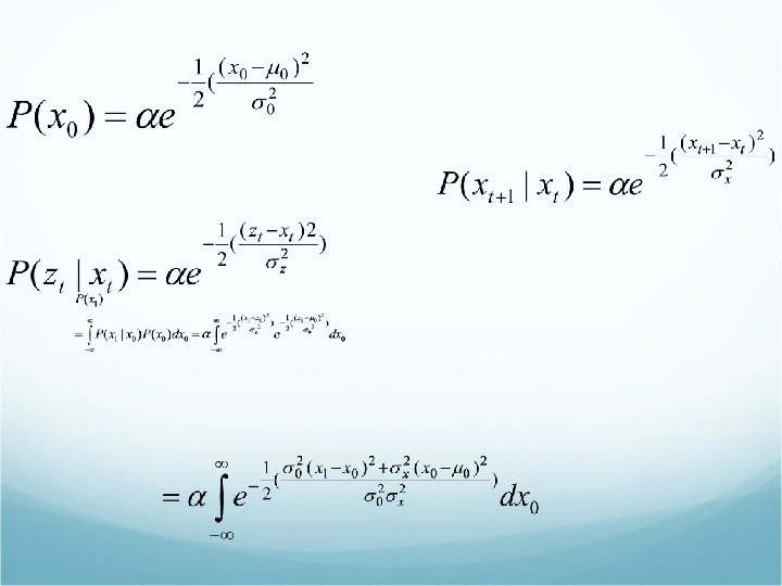
Kalman Filters Linear Gaussian distribution Let X be position be velocity be interval Linear Gaussian transition model with Gaussian noise is:

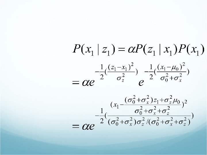
Updating Gaussian distribution If both current distribution P(Xt|e 1: t) and transition model P(Xt+1|xt) are Gaussians then P(Xt+1|e 1: t)= is also Gaussian

If the predicted distribution P(Xt+1|e 1: t) is Gaussian and sensor model P(et+1|Xt+1) is linear Gaussian, then after conditioning on a new evidence, the updated distribution P(Xt+1|e 1: t+1) = α P(et+1|Xt+1) P(Xt+1|e 1: t) is also Gaussian So we could start with a Gaussian prior P(X 0) = N(u 0, Σ 0) and filtering with a linear Gaussian model produces a Gaussian state distribution all the time

Bayesian network for a linear dynamic system Xt Xt+1 Zt Zt+1

ax 02+bx 0+c = a(x 0 -(-b/2 a))2 + c-b 2/4 a

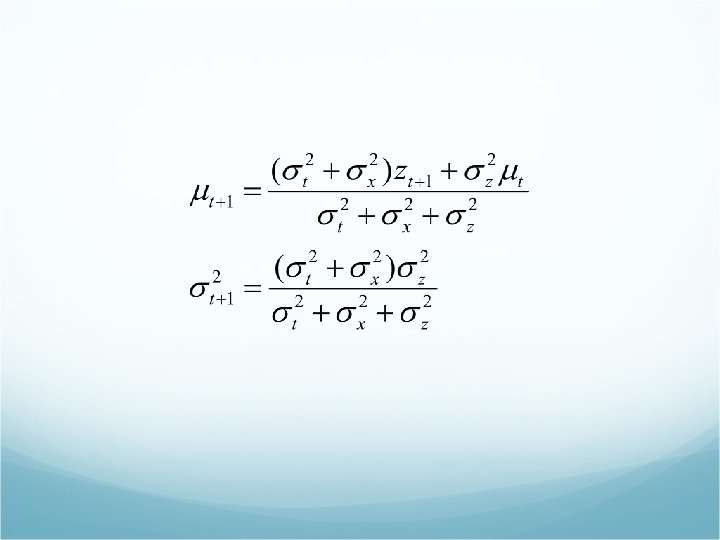
We interpret the calculation for the new mean ut+1 as simply a weighted mean of the new observation zt+1 and old mean ut If the observation is unreliable, then we pay more attention to old mean ut If the old mean ut is unreliable (sigmat is large), or the process is highly unpredictable (sigmax is large), then we pay more attention to observation The sequence of variance values converges to a fixed value that depends on sigmax 2 and sigmaz 2

Extended Kalman Filters The assumptions of a linear Gaussian transition and sensor model are very strong. Extended Kalman filter (EKF) overcomes the nonlineariity. Switching Kalman filter: multi Kalman filters run in parallel, a weighted sum of predictions is used, where weights depends on how well each filter fits the current data. Switching Kalman filter is a special case of Dynamic Bayesian Network (DBN)

Homework 5 Do exercise 15. 2, 15. 6 & 15. 7 Due Dec 24.

Dynamic Belief Networks (DBN) Construction of DBN needs three kinds of information 1. prior distribution P(X 0) 2. transition model P(Xt|Xt-1) 3. the sensor model P(Et|Xt)

Handling failure of sensor If sensor reports “infinity” of object It should imply that the sensor has failed, not that the object has disappeared in an indoor environment

Sensor fusion temperature Sensor model Gauge Reading 1 Gauge reading 2

Transient sensor failure vs persistent sensor failure Battery meter measures might have possibility to fail. Is it battery empty or meter failure?

DBN for robot motion BMeter 1 Battery 0 Battery 1 X’ 0 X’ 1 X 0 X 1 Z 1

Constructing DBN The prior distribution over the state variables P(X 0) The transition model P(Xt+1|Xt) The sensor model P(Et|Xt)

Position Xt , velocity X’t GPS measure of position Zt Sensor model for Bmetert The CPT of P(Bmetert|Batteryt) may contain noise, use Gaussian error model Transient failure vs persistent failure When the robot observes 20 consecutive battery readings of Bmetert=5 but with BMeter 21=0

What will Gaussian error predict about Battery 21? The prediction can use Bayes rule with sensor model P(Bmeter 21=0|Battery 21) and the prediction P(Battery 21|BMeter 1: 20) In order for the system to handle sensor failure properly, the sensor model must include the probability of failure, e. g. P(Bmetert=0|Batteryt=5)=0. 03

Bmeter =5 except t=21, 22 run with Gaussian model E(batteryt) E(Batteryt|… 55500555…) E(Batteryt|… 555000000) 20

Bmeter =5 except t=21, 22 run with transient failure model E(batteryt) E(Batteryt|… 55500555…) E(Batteryt|… 555000000) 20

Adding persistent failure model B 0 P(B 1) t 1. 00 f 0. 001 BMBroken 0 BMBroken 1 E(Batteryt|… 55500555…) 5 E(Batteryt|… 555000000) Bmeter 1 Battery 0 Battery 1 P(BMBrokent|… 55500000… 1 0 P(BMBrokent|… 555005555…)

Exact Inference in DBNs-unrolling a DBN R 0 P(R 1 ) R 1 P(R 2 ) R 2 P(R 3 ) t 0. 7 f 0. 3 Rain 0 Rain 1 P(R 0) Rain 0 Rain 1 Rain 2 Rain 3 Umb 1 Umb 2 Umb 3 P(R 0) 0. 7 Umb 1 R 1 P(U 1 ) t 0. 9 f 0. 2 0. 7 R 1 P(U 1 ) R 2 P(U 2 ) R 3 P(U 3 ) t 0. 9 f 0. 2

Approximate Inference in DBNs Particle sampling: First, a population of N samples is created by sampling from the prior distribution at time 0 P(X 0), then update at each step: Each sample is propagated forward by sampling next state value xt+1 given current value xt for the sample and using the transiiton model P(Xt+1|xt) Each sample is weighted by the likelihood it assigns to the new evidence, P(et+1|xt+1) The population is re-sampled to generate a new population of N samples. Each new sample is selected from the current population; the probability of selection is proportional to its weight. The new samples are unweighted.

Particle Filtering function Particle-Filtering(e, N, dbn) returns a set of samples for the next time step Inputs: e, the new incoming evidence N, the number of samples to be maintained Dbn, a DBN with prior P(X 0), transition model P(X 1|X 0), the sensor model P(E 1|X 1) static: S, a vector of samples of size N, initially generated from P(X 0) local variables: W, a vector of weights of size N For i =1 to N do S[i] ← sample from P(X 1|X 0 = S[i]) W[i] ← P(e|X 1=S[i]) S ← WEIGHTED-SMAPLE-WITH-REPALCEMENT(N, S, W) Return S

Is particle sampling consistent and efficient? Consistency: Particle sampling is consistent as N tends to infinity. The number of samples occupying xt after observing e 1: t N(xt|e 1: t)/N = P(xt|e 1: t) The number of reach xt+1 is N(xt+1|e 1: t) = ∑xt. P(xt+1|xt) N(xt|e 1: t)

Weighting each sample by its likelihood for the evidence at t+1: W(xt+1|e 1: t) = P(et+1|xt+1)N(xt+1|e 1: t) Now resample with probability proportional to its weights, the number of samples in state xt+1 after resampling is proportional to the total weight in xt+1 before resampling: N(xt+1|e 1: t+1)/N = α W(xt+1|e 1: t+1) = α P(et+1|xt+1)N(xt+1|e 1: t) = αP(et+1|xt+1) ∑xt. P(xt+1|xt) N(xt|e 1: t) = αN P(et+1|xt+1) ∑xt. P(xt+1|xt) P(xt|e 1: t) = P(xt+1|e 1: t+1)

Efficiency Particle sampling seems to maintain a good approximation to the true posterior using a constant number of smaples. There are, as yet, no theoretical guarantees; particle filtering is currently an area of intensive study.

Outline Probability theory Bayesian Belief network Ø Decision Theoretic Reasoning Sequential Decision theoretic reasoning

Utility theory Lottery L=[p, A; 1 -p, B] Preference over lotteries or uncertain states A B A~B A B The degree of preference over states can be expressed in terms of a utility function that maps the state into a real number U(A)

Axioms of utility theory Orderability: (A >B) (B>A) (A~B) Transitivity: (A>B) (B>C) (A>C) Continuity: A>B>C p [p, A; 1 -p, C]~B Substitutability: A~B [p, A; 1 -p, C]~[p, B; 1 -p, C] Monotonicity: A>B (p q [p, A; 1 -p; B] [q, A; 1 q, B] Decomposability: [p, A; 1 -p, [q, B; 1 -q, C]]~ [p, A; (1 -p)q, B; (1 -p)(1 -q), C]

Utility principle U(A) > U(B) A >B U(A)=U(B) A~B Maximum expected utility principle U([p 1, S 1; …, pn, Sn])= i pi. U(Si)

Utility of money $1, 000 prize is awarded to you or if you would accept a gamble of $3, 000 determined by flipping a coin (Head: win, Tail: nothing) The expected monetary value (EMV) is $1, 500, 000

Expected monetary value Sn denote the state of possessing total wealth $n and $k is the current wealth EU(Accept)=1. 2 U(Sk)+1/2 U(Sk+3, 000) EU(Decline)=U(Sk+1000, 000)

St. Petersburg Paradox [1738] If the head appear at the n-th toss, you win 2 n dollars. EMV(St. P. ) = i P(Headsi)MV(Heads) = i (1/2 i) 2 i=2/2+4/4+8/8+…= You should bet infinite amount?

Bernoulli’s logarithmic utility Bernoulli proposed logarithmic utility of money U(Sk+n)=log 2 n (for n > 0) EU(St. P. )= i P(Headsi)U(Headsi) = i (1/2 i) log 22 i = ½ + 2/4 + 3/8 + …= 2 So a rational agent will pay up to $4.

Risk preference Risk averse: prefer a sure thing with a payoff less than the expected monetary payoff Risk neutral: equal to Risk seeking: greater than Certainty equivalent: the value an agent accept in lieu of a lottery Insurance premium: the difference between the expected monetary payoff of a lottery and its certainty equivalent

Definition of risk preference Risk averse: Risk neutral: Risk seeking:

Risk Preference Types Risk averse Utility u(x) Risk seeking Risk neutral Monetary payoff x

Utility functions of different risk attitudes Risk neutral u(x)=x Risk averse u(x)= x Risk seeking u(x)=x 2

Certainty equivalent The value an agent will accept in lieu of a lottery The difference between the expected money value of a lottery and its certainty equivalent is called insurance premium

Human judgment A: 80% 4000 C: 20% 4000 B: 100% 3000 D: 25% 3000

Majority decision B>A ; C>D 0. 8 U($4000) <U($3000) 0. 2 U($4000)>0. 25 U($3000) No utility function could satisfy the preference One explanation of this is to take regret into account

Multi-attribute Utility Function U(x 1, . . , xn)=f(f 1(x 1), …, fn(xn)) dominance X 2 C B A D X 1 A is strictly dominated by B

Stochastic dominance x - xp 1(x’)dx’ - xp 2(x’)dx’ S 1 stochastically dominates S 2 S 1

Decision Networks Chance node Decision node Utility node Airport Site Air Traffic deaths Litigation noise Construction Cost U

Value of Information Value of perfect information EU( |E) = max. A i. U(Resulti(A))P(Resulti(A)|E, Do(A)) EU( Ej|E, Ej) = max. A i. U(Resulti(A))P(Resulti(A)|E, Do(A), Ej) VPIE(Ej)=( P(Ej=ejk|E)EU( ejk|E, Ej=ejk))-EU( |E)

Information Gathering Agents Function Information. Gathering. Agent(percept) returns an action Static: D, a decision network Integrate percept into D J the value that maxmize VPI(Ej)-cost(Ej) If VPI(Ej) > Cost(Ej) the return Request(Ej) Else return the best action from D

Properties Of Value of Information j, E VPIE(Ej) 0 VPIE(Ej, Ek) VPIE(Ej)+VPIE(Ek) Order independent: VPIE(Ej, Ek) = VPIE(Ej)+VPIE, Ej(Ek) =VPIE(Ek)+VPIE, Ek(Ej)

Dynamic Decision Networks Add utility nodes and decision nodes for actions in DBN

Decision-theoretic agent Function Decision-theoretic-agent(percept) return action Calculate updated probabilities for current state based on available evidence including current percept and previous action Calculate outcome probabilities for actions given action descriptions and probabilities of current state Select action with highest expected utility given probabilities of outcomes and utility information Return action

Partially Observable MDP POMDP belief state b(s) is updated b’(s’) = O(s’, o) s. T(s, a, s’)b(s) P(o|a, b) = s’P(o|a, s’, b)P(s’|a, b) = s’O(s’, o) s. T(s, a, s’)b(s)

Decision Theoretic Agents The transition and observation models are represented by a dynamic Bayesian network. The dynamic Bayesian network is extended with decision and utility nodes as in decision networks. The resulting model is called dynamic decision network DDN. A filtering algorithm is used to incorporate each new percept and action and to update the belief state representation. Decision are made by projecting possible action sequence and choosing the best one.

Decision theoretic Agent Function Decision-Theoretic-Agent(Et) return an action inputs: Et, the percept at time t static BN, a belief network with nodes X Bel(X), a vector of probabilities, updated over time Bel(Xt) Xt-1 P(Xt|Xt-1= xt-1, At-1) Bel(Xt-1= xt-1 ) Bel(Xt) P(Et|Xt) Bel(Xt) action arg max. At xt[Bel(Xt) xt+1 P(Xt+1 = xt+1 |Xt= xt , At) U(xt+1 )] Return action