Chapter 13 Multiple Regression 1 Chapter Outline Multiple

Chapter 13 Multiple Regression 1

Chapter Outline Ø Multiple Regression Model Ø Least Squares Method Ø Coefficient of Determination Ø Model Assumptions Ø Testing for Significance Ø Estimation and Prediction Ø Categorical Independent Variables 2

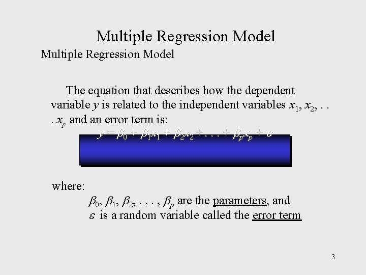
Multiple Regression Model The equation that describes how the dependent variable y is related to the independent variables x 1, x 2, . . . xp and an error term is: y = 0 + 1 x 1 + 2 x 2 +. . . + pxp + where: 0, 1, 2, . . . , p are the parameters, and is a random variable called the error term 3

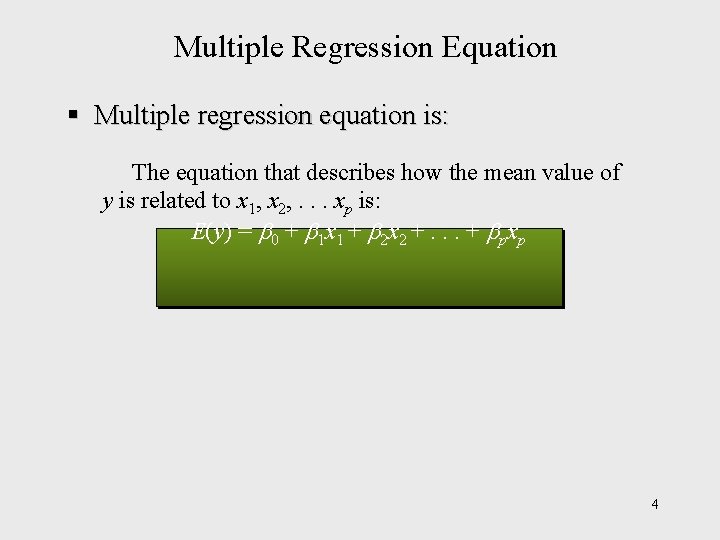
Multiple Regression Equation § Multiple regression equation is: The equation that describes how the mean value of y is related to x 1, x 2, . . . xp is: E(y) = 0 + 1 x 1 + 2 x 2 +. . . + pxp 4

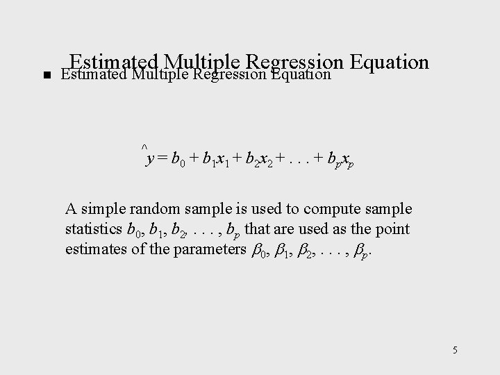
n Estimated Multiple Regression Equation ^ y = b 0 + b 1 x 1 + b 2 x 2 +. . . + bpxp A simple random sample is used to compute sample statistics b 0, b 1, b 2, . . . , bp that are used as the point estimates of the parameters 0, 1, 2, . . . , p. 5

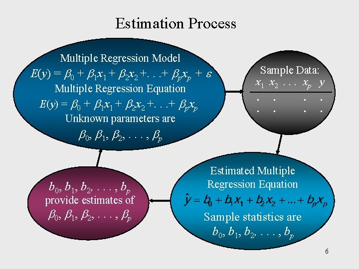
Estimation Process Multiple Regression Model E(y) = 0 + 1 x 1 + 2 x 2 +. . . + pxp + Multiple Regression Equation E(y) = 0 + 1 x 1 + 2 x 2 +. . . + pxp Unknown parameters are Sample Data: x 1 x 2. . . xp y. . . . 0, 1, 2, . . . , p b 0, b 1, b 2, . . . , bp Estimated Multiple Regression Equation provide estimates of 0, 1, 2, . . . , p Sample statistics are b 0, b 1, b 2, . . . , bp 6

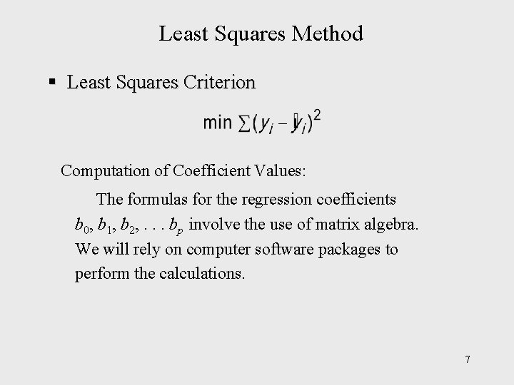
Least Squares Method § Least Squares Criterion Computation of Coefficient Values: The formulas for the regression coefficients b 0, b 1, b 2, . . . bp involve the use of matrix algebra. We will rely on computer software packages to perform the calculations. 7

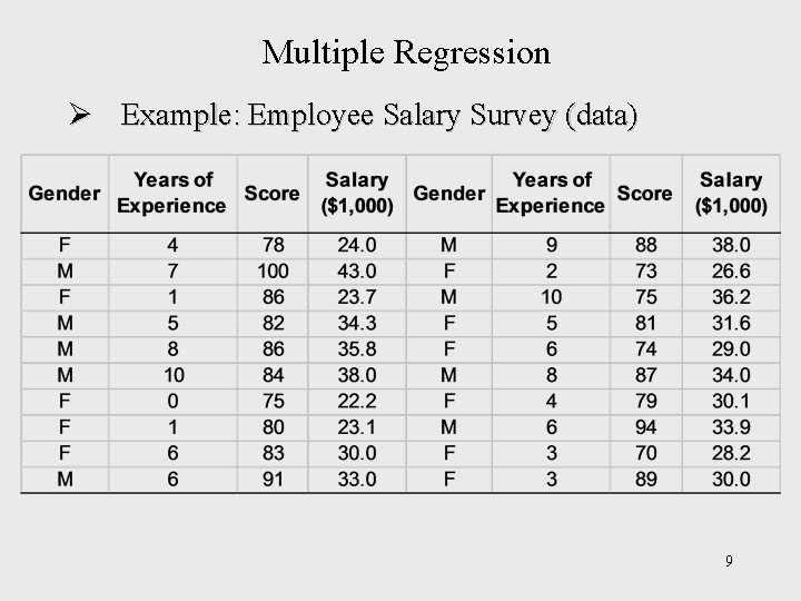
Multiple Regression Ø Example: Employee Salary Survey A local firm collected data for a sample of 20 employees. A suggestion was made that regression analysis could be used to determine if salary was related to the years of experience and the score on the firm’s aptitude test. The gender of employees, years of experience, score on the aptitude test, and corresponding annual salary ($1000 s) for a sample of 20 employees is shown on the next slide. 8

Multiple Regression Ø Example: Employee Salary Survey (data) 9

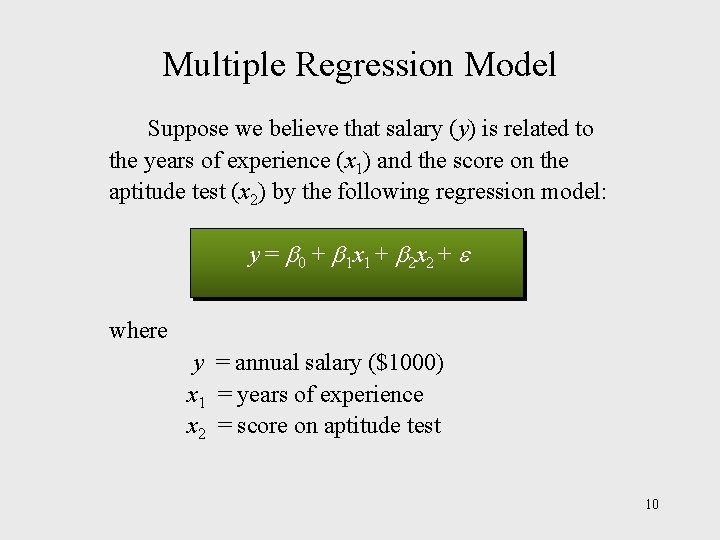
Multiple Regression Model Suppose we believe that salary (y) is related to the years of experience (x 1) and the score on the aptitude test (x 2) by the following regression model: y = 0 + 1 x 1 + 2 x 2 + where y = annual salary ($1000) x 1 = years of experience x 2 = score on aptitude test 10

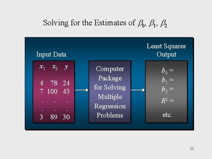
Solving for the Estimates of 0, 1, 2 Least Squares Output Input Data x 1 x 2 y 4 78 24 7 100 43. . . 3 89 30 Computer Package for Solving Multiple Regression Problems b 0 = b 1 = b 2 = R 2 = etc. 11

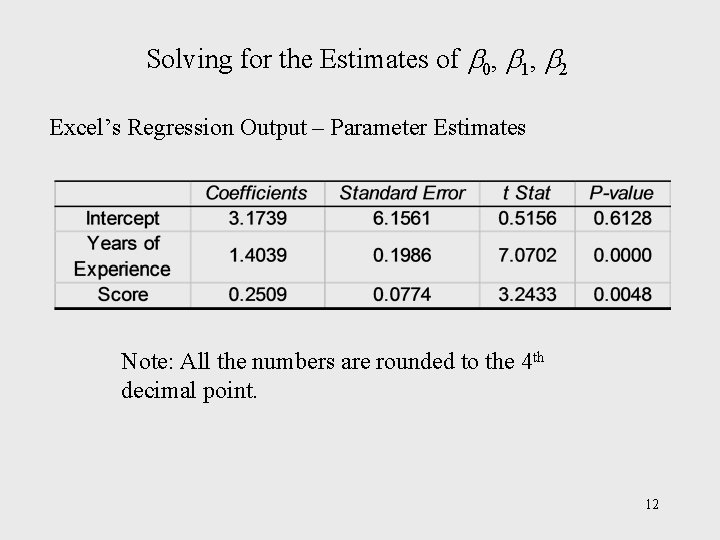
Solving for the Estimates of 0, 1, 2 Excel’s Regression Output – Parameter Estimates Note: All the numbers are rounded to the 4 th decimal point. 12

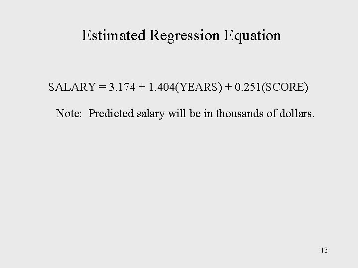
Estimated Regression Equation SALARY = 3. 174 + 1. 404(YEARS) + 0. 251(SCORE) Note: Predicted salary will be in thousands of dollars. 13

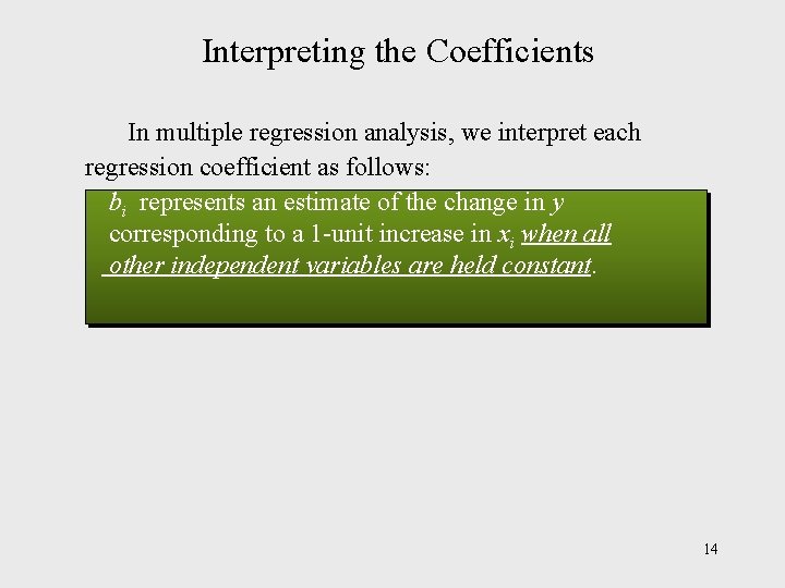
Interpreting the Coefficients In multiple regression analysis, we interpret each regression coefficient as follows: bi represents an estimate of the change in y corresponding to a 1 -unit increase in xi when all other independent variables are held constant. 14

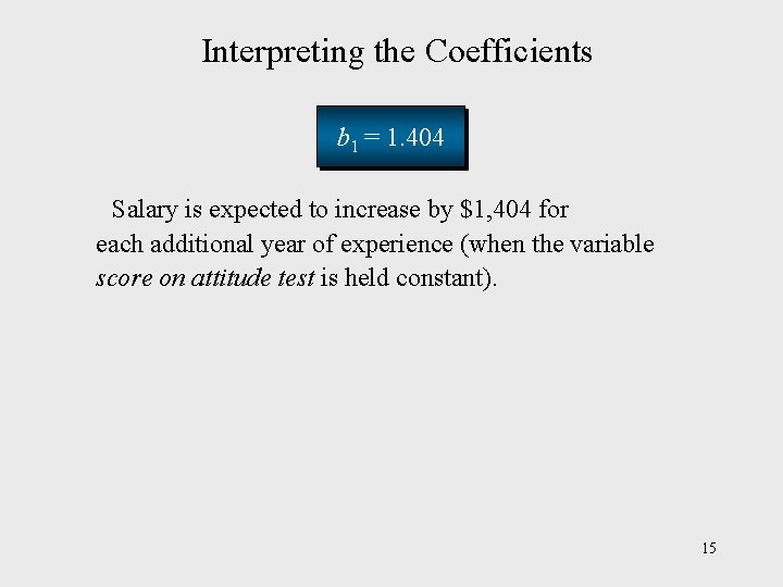
Interpreting the Coefficients b 1 = 1. 404 Salary is expected to increase by $1, 404 for each additional year of experience (when the variable score on attitude test is held constant). 15

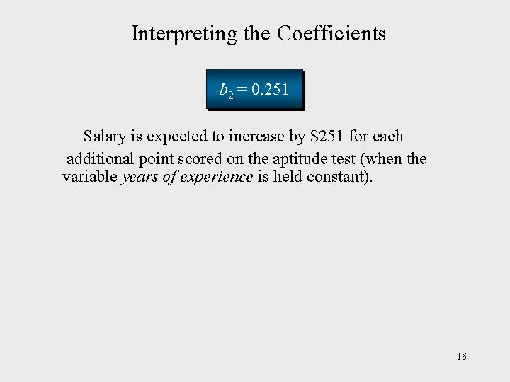
Interpreting the Coefficients b 2 = 0. 251 Salary is expected to increase by $251 for each additional point scored on the aptitude test (when the variable years of experience is held constant). 16

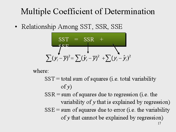
Multiple Coefficient of Determination • Relationship Among SST, SSR, SSE SST SSE = SSR + where: SST = total sum of squares (i. e. total variability of y) SSR = sum of squares due to regression (i. e. the variability of y that is explained by regression) SSE = sum of squares due to error (i. e. the variability of y that cannot be explained by regression) 17

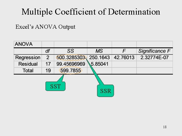
Multiple Coefficient of Determination Excel’s ANOVA Output SST SSR 18

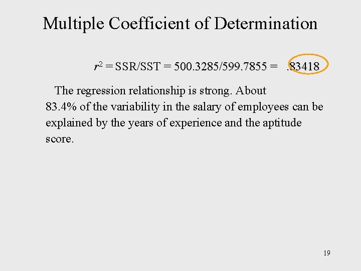
Multiple Coefficient of Determination r 2 = SSR/SST = 500. 3285/599. 7855 =. 83418 The regression relationship is strong. About 83. 4% of the variability in the salary of employees can be explained by the years of experience and the aptitude score. 19

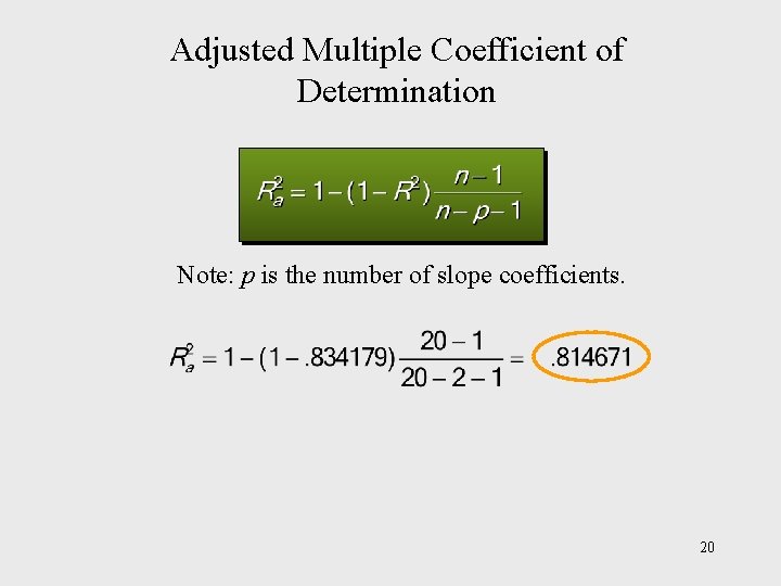
Adjusted Multiple Coefficient of Determination Note: p is the number of slope coefficients. 20

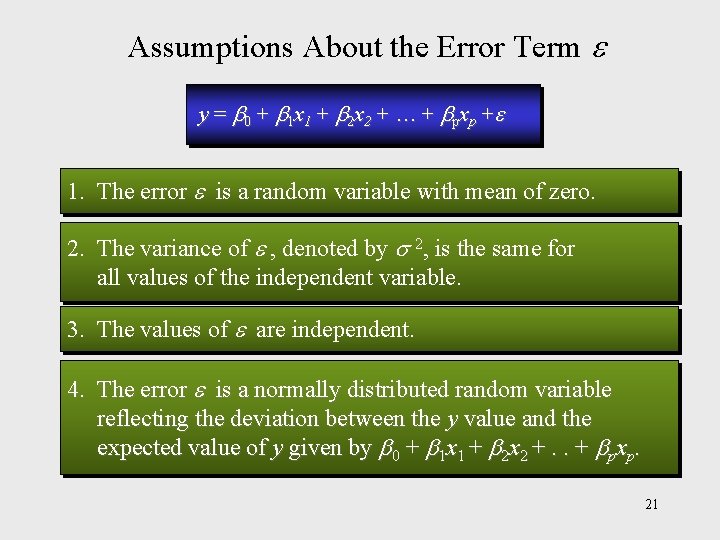
Assumptions About the Error Term y = 0 + 1 x 1 + 2 x 2 + … + pxp + 1. The error is a random variable with mean of zero. 2. The variance of , denoted by 2, is the same for all values of the independent variable. 3. The values of are independent. 4. The error is a normally distributed random variable reflecting the deviation between the y value and the expected value of y given by 0 + 1 x 1 + 2 x 2 +. . + pxp. 21

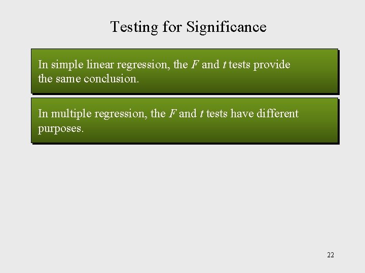
Testing for Significance In simple linear regression, the F and t tests provide the same conclusion. In multiple regression, the F and t tests have different purposes. 22

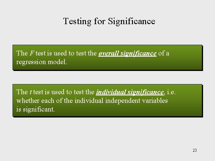
Testing for Significance The F test is used to test the overall significance of a regression model. The t test is used to test the individual significance, i. e. whether each of the individual independent variables is significant. 23

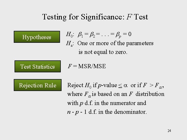
Testing for Significance: F Test Hypotheses H 0: 1 = 2 =. . . = p = 0 Ha: One or more of the parameters is not equal to zero. Test Statistics F = MSR/MSE Rejection Rule Reject H 0 if p-value < a or if F > F , where F is based on an F distribution with p d. f. in the numerator and n - p - 1 d. f. in the denominator. 24

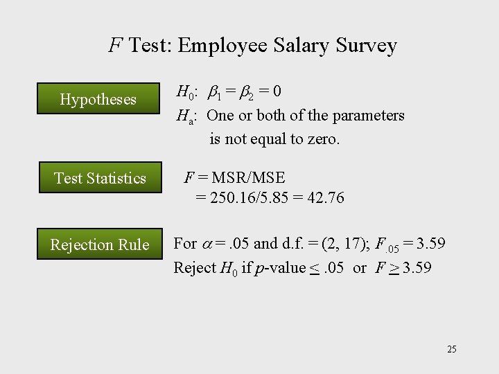
F Test: Employee Salary Survey Hypotheses Test Statistics Rejection Rule H 0: 1 = 2 = 0 Ha: One or both of the parameters is not equal to zero. F = MSR/MSE = 250. 16/5. 85 = 42. 76 For =. 05 and d. f. = (2, 17); F. 05 = 3. 59 Reject H 0 if p-value <. 05 or F > 3. 59 25

F Test: Employee Salary Survey p-value Conclusion p-value <. 05, so we can reject H 0. (Also, F = 42. 76 > 3. 59) 26

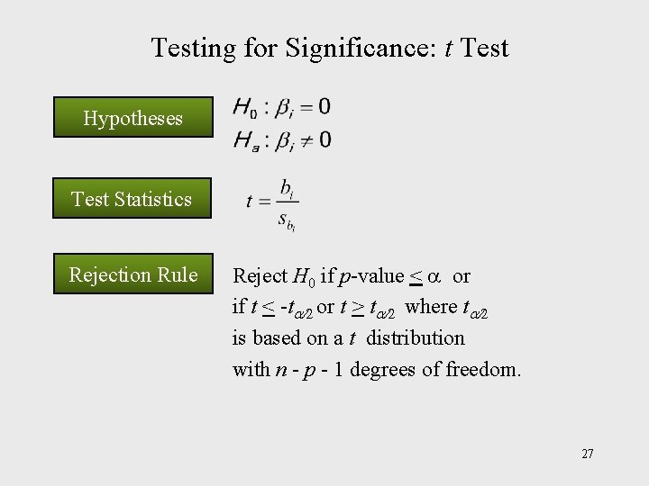
Testing for Significance: t Test Hypotheses Test Statistics Rejection Rule Reject H 0 if p-value < a or if t < -t or t > t where t is based on a t distribution with n - p - 1 degrees of freedom. 27

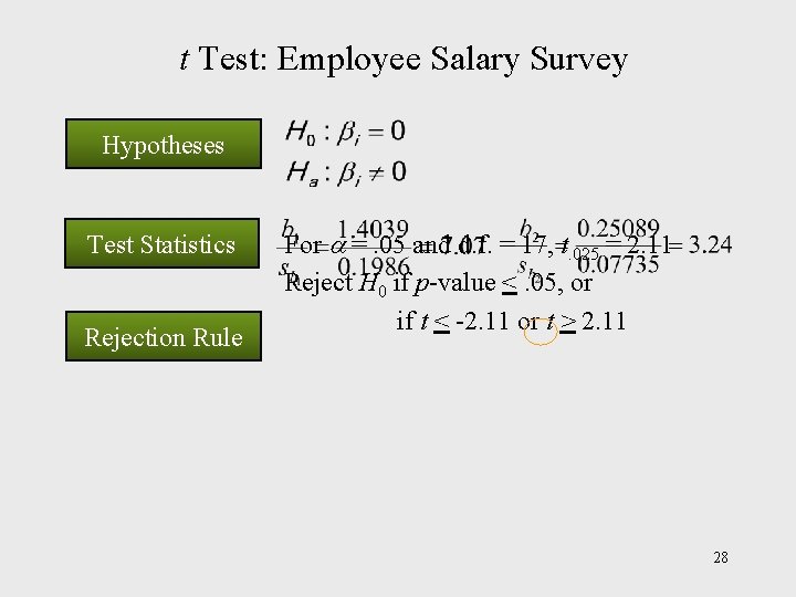
t Test: Employee Salary Survey Hypotheses Test Statistics Rejection Rule For =. 05 and d. f. = 17, t. 025 = 2. 11 Reject H 0 if p-value <. 05, or if t < -2. 11 or t > 2. 11 28

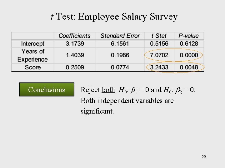
t Test: Employee Salary Survey Conclusions Reject both H 0: 1 = 0 and H 0: 2 = 0. Both independent variables are significant. 29

Test for Significance: Multicollinearity The term multicollinearity refers to the correlation among the independent variables. When the independent variables are highly correlated (say, |r | >. 7), it is not possible to determine the separate effect of any particular independent variable on the dependent variable. 30

Using the Estimated Regression Equation for Estimation and Prediction The procedures for estimating the mean value of y and predicting an individual value of y in multiple regression are similar to those in simple regression. We substitute the given values of x 1, x 2, . . . , xp into the estimated regression equation and use the corresponding value of y as the point estimate. 31

Categorical Independent Variables In many situations we must work with categorical independent variables such as gender (male, female), method of payment (cash, check, credit card), etc. For example, xi might represent gender where xi = 0 indicates male and xi = 1 indicates female. In this case, xi is called a dummy or indicator variable. 32

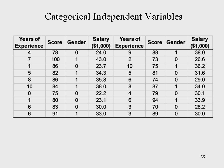
Categorical Independent Variables Example: Employee Salary Survey As an extension of the problem involving the employee salary survey, suppose that management wants to find out if the annual salary is related to employees’ gender. The years of experience, the score on the aptitude test, employees’ gender, and the annual salary ($000) for each of the sampled 20 employees are shown on the next slide. 33

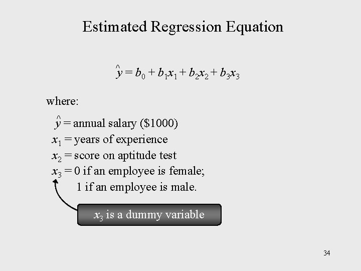
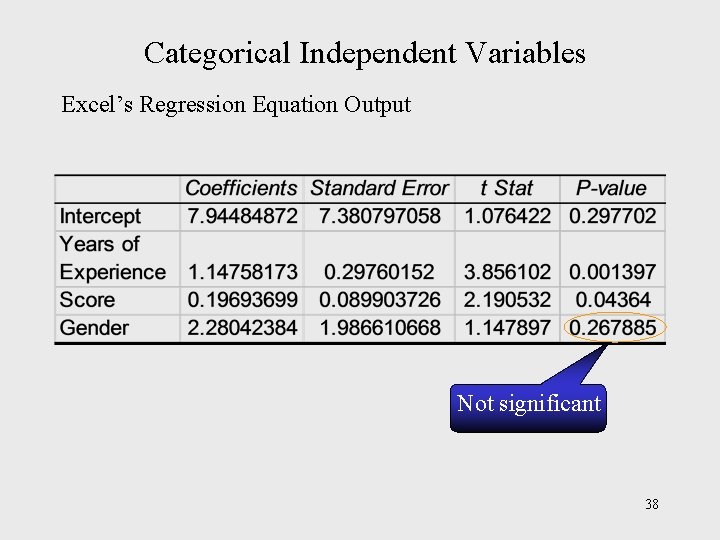
Estimated Regression Equation ^ y = b 0 + b 1 x 1 + b 2 x 2 + b 3 x 3 where: y^ = annual salary ($1000) x 1 = years of experience x 2 = score on aptitude test x 3 = 0 if an employee is female; 1 if an employee is male. x 3 is a dummy variable 34

Categorical Independent Variables 35

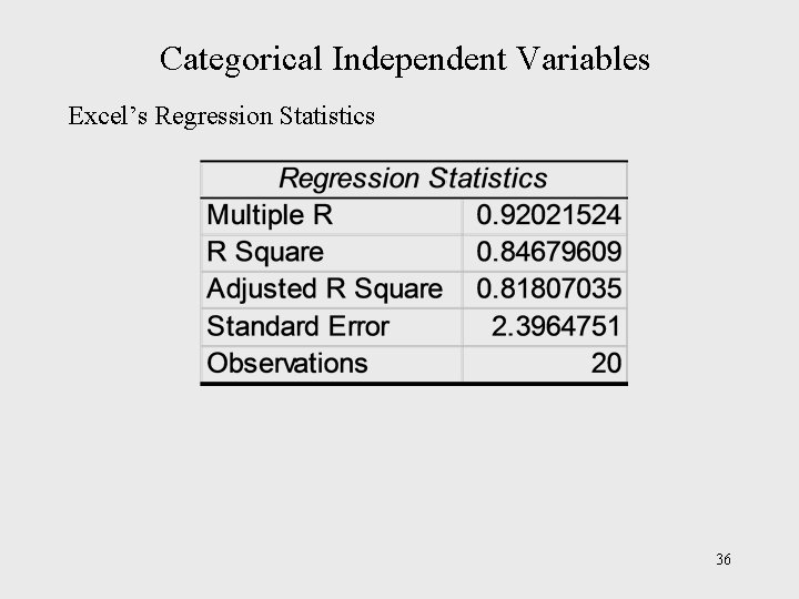
Categorical Independent Variables Excel’s Regression Statistics 36

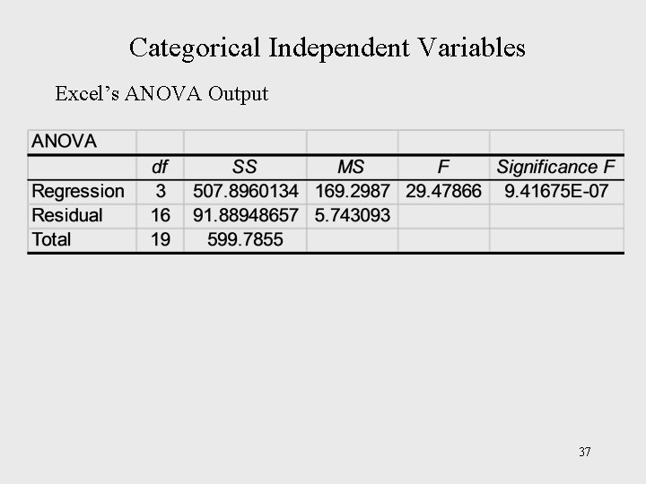
Categorical Independent Variables Excel’s ANOVA Output 37

Categorical Independent Variables Excel’s Regression Equation Output Not significant 38