Multiple Regression Multiple regression Typically we want to

Multiple Regression

Multiple regression Typically, we want to use more than a single predictor (independent variable) to make predictions Regression with more than one predictor is called “multiple regression”

Motivating example: Sex discrimination in wages In 1970’s, Harris Trust and Savings Bank was sued for discrimination on the basis of sex. Analysis of salaries of employees of one type (skilled, entry-level clerical) presented as evidence by the defense. Did female employees tend to receive lower starting salaries than similarly qualified and experienced male employees?

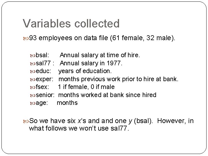
Variables collected 93 employees on data file (61 female, 32 male). bsal: sal 77 : educ: exper: fsex: senior: age: Annual salary at time of hire. Annual salary in 1977. years of education. months previous work prior to hire at bank. 1 if female, 0 if male months worked at bank since hired months So we have six x’s and one y (bsal). However, in what follows we won’t use sal 77.

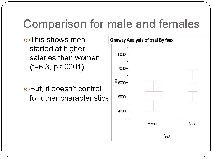
Comparison for male and females This shows men started at higher salaries than women (t=6. 3, p<. 0001). But, it doesn’t control for other characteristics.

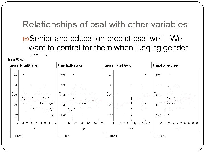
Relationships of bsal with other variables Senior and education predict bsal well. We want to control for them when judging gender effect.

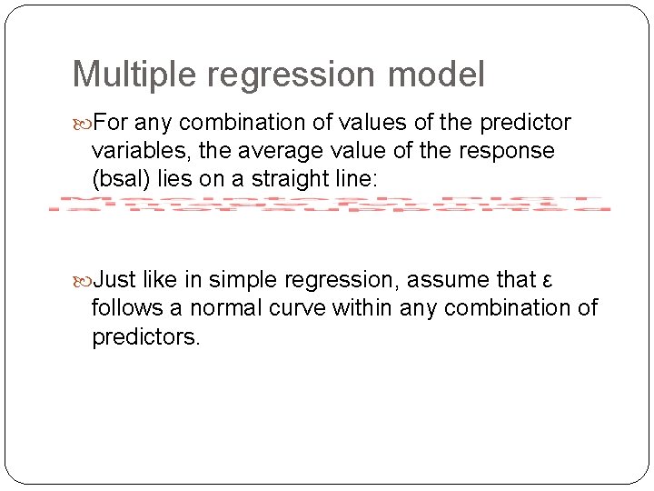
Multiple regression model For any combination of values of the predictor variables, the average value of the response (bsal) lies on a straight line: Just like in simple regression, assume that ε follows a normal curve within any combination of predictors.

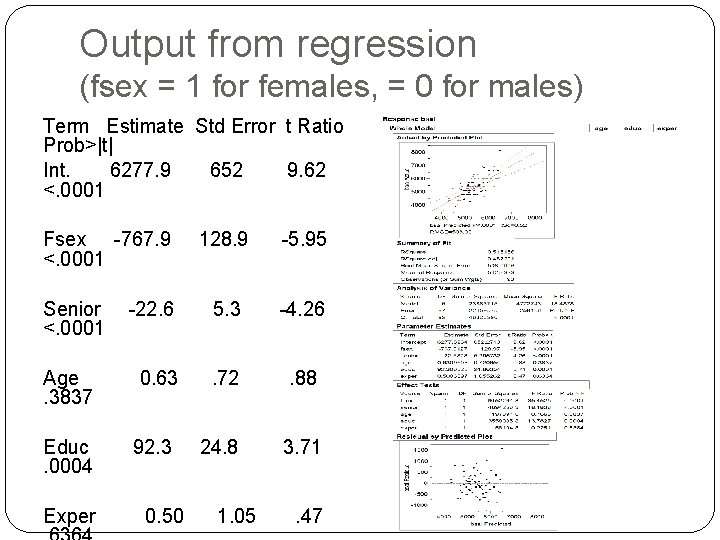
Output from regression (fsex = 1 for females, = 0 for males) Term Estimate Std Error t Ratio Prob>|t| Int. 6277. 9 652 9. 62 <. 0001 Fsex -767. 9 <. 0001 Senior <. 0001 Age. 3837 Educ. 0004 Exper 128. 9 -5. 95 -22. 6 5. 3 -4. 26 0. 63 . 72 . 88 24. 8 3. 71 92. 3 0. 50 1. 05 . 47

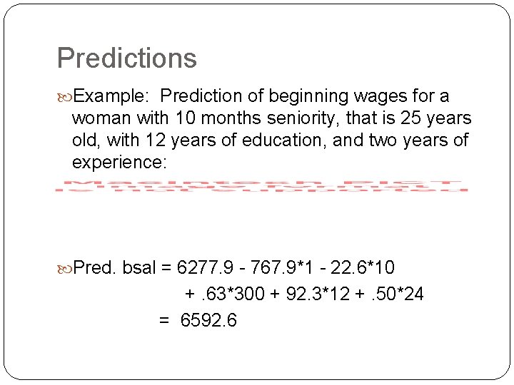
Predictions Example: Prediction of beginning wages for a woman with 10 months seniority, that is 25 years old, with 12 years of education, and two years of experience: Pred. bsal = 6277. 9 - 767. 9*1 - 22. 6*10 +. 63*300 + 92. 3*12 +. 50*24 = 6592. 6

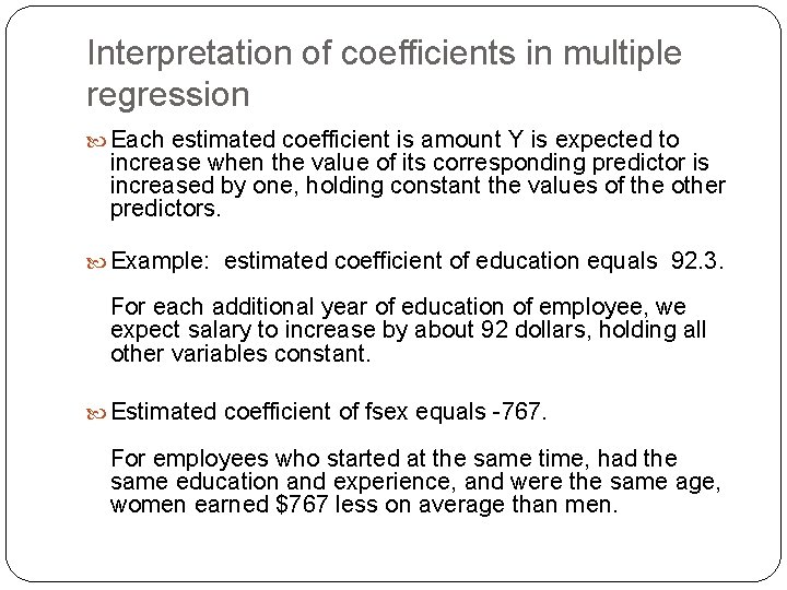
Interpretation of coefficients in multiple regression Each estimated coefficient is amount Y is expected to increase when the value of its corresponding predictor is increased by one, holding constant the values of the other predictors. Example: estimated coefficient of education equals 92. 3. For each additional year of education of employee, we expect salary to increase by about 92 dollars, holding all other variables constant. Estimated coefficient of fsex equals -767. For employees who started at the same time, had the same education and experience, and were the same age, women earned $767 less on average than men.

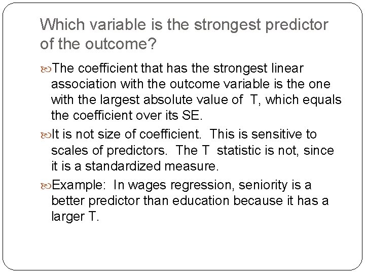
Which variable is the strongest predictor of the outcome? The coefficient that has the strongest linear association with the outcome variable is the one with the largest absolute value of T, which equals the coefficient over its SE. It is not size of coefficient. This is sensitive to scales of predictors. The T statistic is not, since it is a standardized measure. Example: In wages regression, seniority is a better predictor than education because it has a larger T.

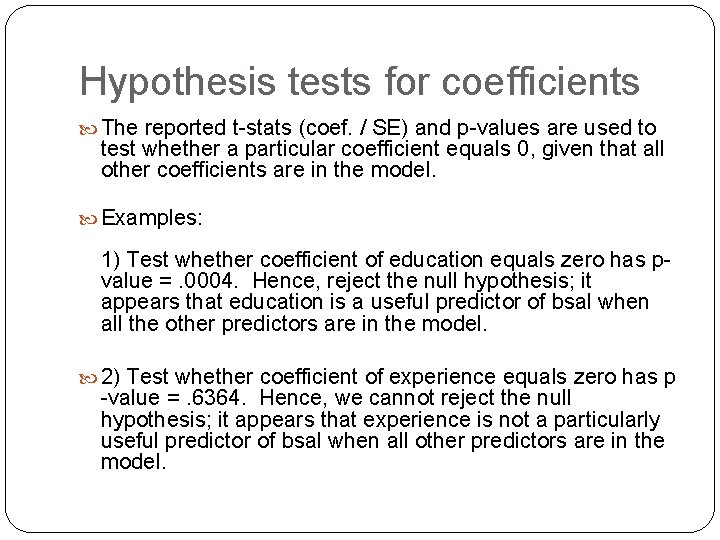
Hypothesis tests for coefficients The reported t-stats (coef. / SE) and p-values are used to test whether a particular coefficient equals 0, given that all other coefficients are in the model. Examples: 1) Test whether coefficient of education equals zero has pvalue =. 0004. Hence, reject the null hypothesis; it appears that education is a useful predictor of bsal when all the other predictors are in the model. 2) Test whether coefficient of experience equals zero has p -value =. 6364. Hence, we cannot reject the null hypothesis; it appears that experience is not a particularly useful predictor of bsal when all other predictors are in the model.

Hypothesis tests for coefficients The test statistics have the usual form (observed – expected)/SE. For p-value, use area under a t-curve with (n-k) degrees of freedom, where k is the number of terms in the model. In this problem, the degrees of freedom equal (93 -6=87).

CIs for regression coefficients A 95% CI for the coefficients is obtained in the usual way: coef. ± (multiplier) SE The multiplier is obtained from the t-curve with (n-k) degrees of freedom. (If degrees of freedom is greater than 26 use normal table) Example: A 95% CI for the population regression coefficient of age equals: (0. 63 – 1. 96*0. 72, 0. 63 + 1. 96*0. 72)

Warning about tests and CIs Hypothesis tests and CIs are meaningful only when the data fits the model well. Remember, when the sample size is large enough, you will probably reject any null hypothesis of β=0. When the sample size is small, you may not have enough evidence to reject a null hypothesis of β=0. When you fail to reject a null hypothesis, don’t be too hasty to say that a predictor has no linear association with the outcome. It is likely that there is some association, it just isn’t a very strong one.

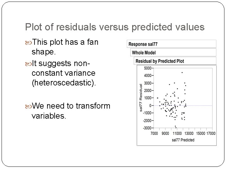
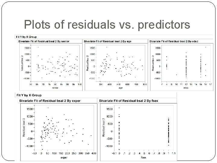
Checking assumptions Plot the residuals versus the predicted values from the regression line. Also plot the residuals versus each of the predictors. If non-random patterns in these plots, the assumptions might be violated.

Plot of residuals versus predicted values This plot has a fan shape. It suggests nonconstant variance (heteroscedastic). We need to transform variables.

Plots of residuals vs. predictors

Summary of residual plots There appears to be a non-random pattern in the plot of residuals versus experience, and also versus age. This model can be improved.

Modeling categorical predictors When predictors are categorical and assigned numbers, regressions using those numbers make no sense. Instead, we make “dummy variables” to stand in for the categorical variables.

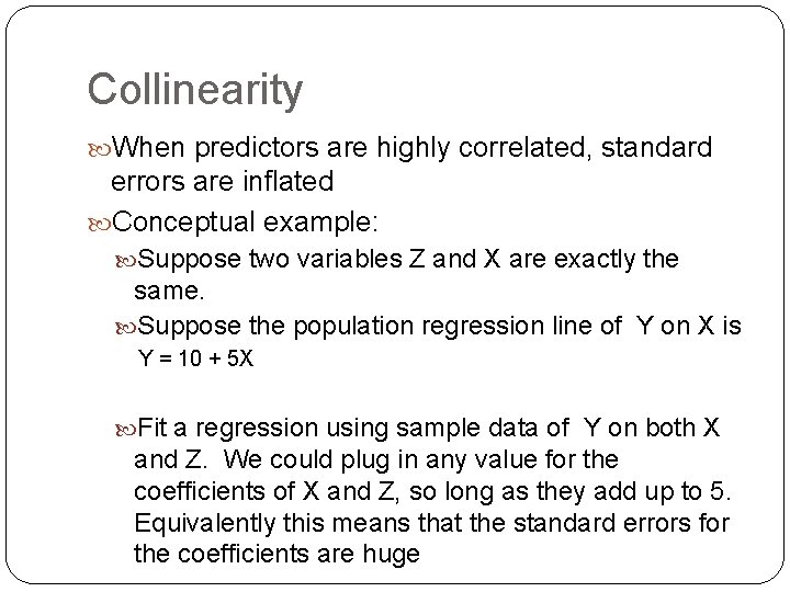
Collinearity When predictors are highly correlated, standard errors are inflated Conceptual example: Suppose two variables Z and X are exactly the same. Suppose the population regression line of Y on X is Y = 10 + 5 X Fit a regression using sample data of Y on both X and Z. We could plug in any value for the coefficients of X and Z, so long as they add up to 5. Equivalently this means that the standard errors for the coefficients are huge

General warnings for multiple regression Be even more wary of extrapolation. Because there are several predictors, you can extrapolate in many ways Multiple regression shows association. It does not prove causality. Only a carefully designed observational study or randomized experiment can show causality