Multiple Regression Anal Let us start with Simple

Multiple Regression Anal

Let us start with Simple Linear Regression

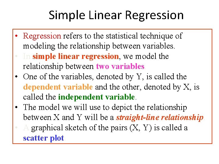
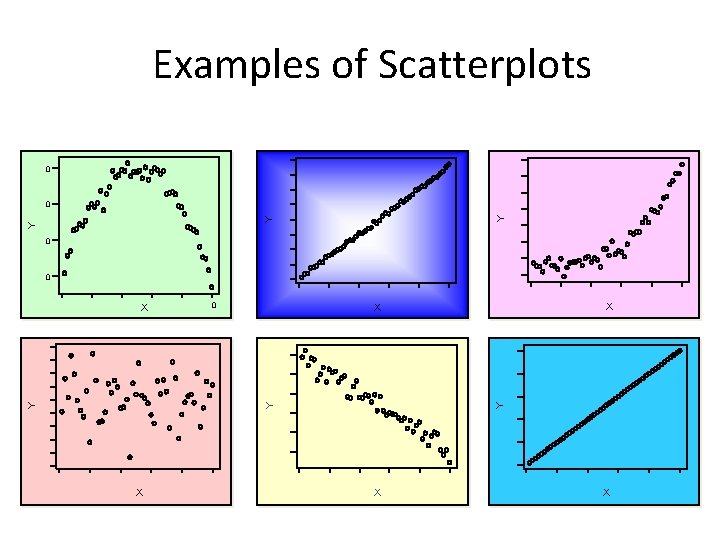
Simple Linear Regression • Regression refers to the statistical technique of modeling the relationship between variables. • In simple linear regression, regression we model the relationship between two variables • One of the variables, denoted by Y, is called the dependent variable and the other, denoted by X, is called the independent variable • The model we will use to depict the relationship between X and Y will be a straight-line relationship • A graphical sketch of the pairs (X, Y) is called a scatter plot

Examples of Scatterplots 0 Y Y Y 0 0 X X X Y Y Y X X X

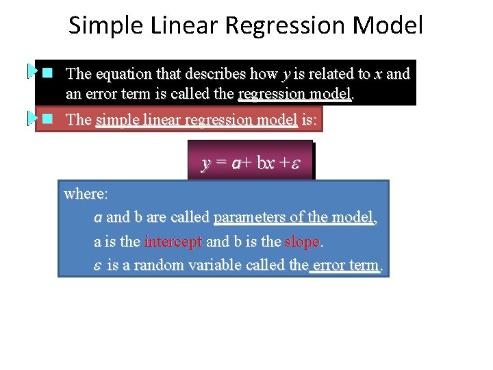
Simple Linear Regression Model n The equation that describes how y is related to x and an error term is called the regression model. n The simple linear regression model is: y = a+ b x + e where: a and b are called parameters of the model, a is the intercept and b is the slope. e is a random variable called the error term.

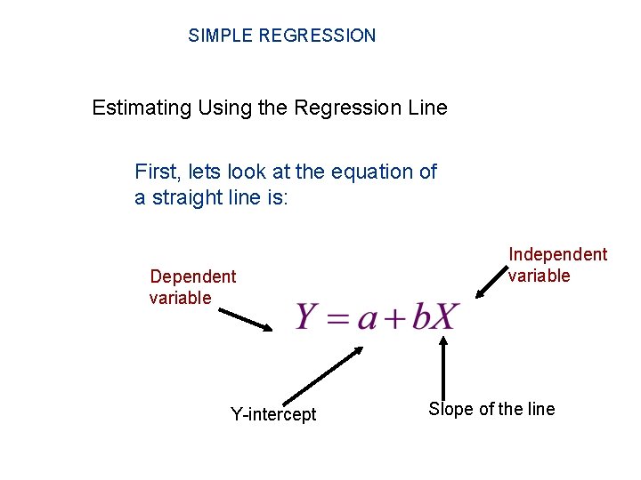
SIMPLE REGRESSION Estimating Using the Regression Line First, lets look at the equation of a straight line is: Dependent variable Y-intercept Independent variable Slope of the line

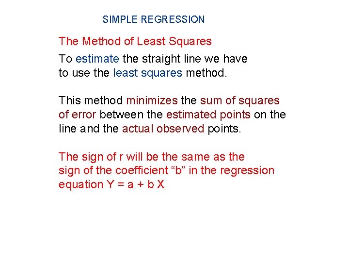
SIMPLE REGRESSION The Method of Least Squares To estimate the straight line we have to use the least squares method. This method minimizes the sum of squares of error between the estimated points on the line and the actual observed points. The sign of r will be the same as the sign of the coefficient “b” in the regression equation Y = a + b X

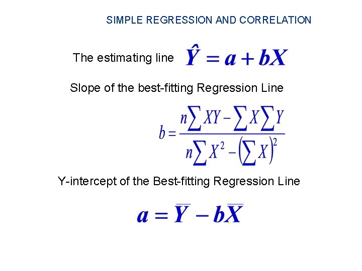
SIMPLE REGRESSION AND CORRELATION The estimating line Slope of the best-fitting Regression Line Y-intercept of the Best-fitting Regression Line

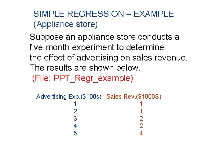
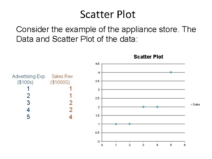
SIMPLE REGRESSION – EXAMPLE (Appliance store) Suppose an appliance store conducts a five-month experiment to determine the effect of advertising on sales revenue. The results are shown below. (File: PPT_Regr_example) Advertising Exp. ($100 s) Sales Rev. ($1000 S) 1 1 2 1 3 2 4 2 5 4

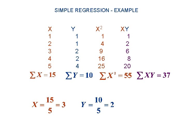
SIMPLE REGRESSION - EXAMPLE X 1 2 3 4 5 Y 1 1 2 2 4 X 2 1 4 9 16 25 XY 1 2 6 8 20

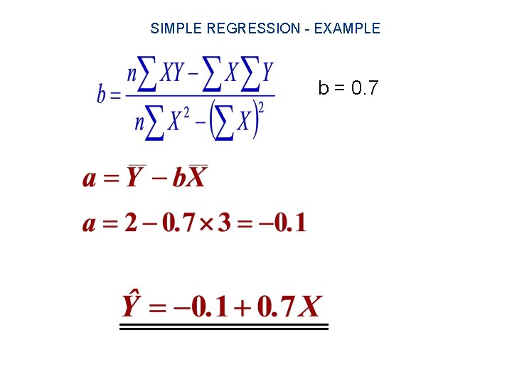
SIMPLE REGRESSION - EXAMPLE b = 0. 7

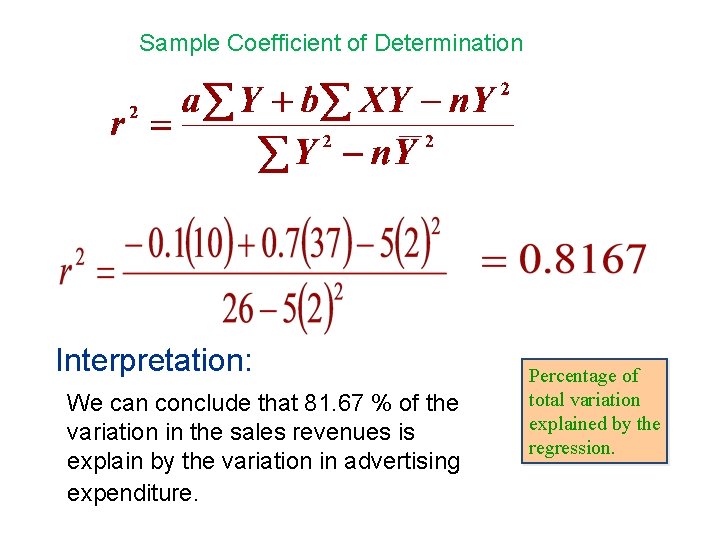
Sample Coefficient of Determination Interpretation: We can conclude that 81. 67 % of the variation in the sales revenues is explain by the variation in advertising expenditure. Percentage of total variation explained by the regression.

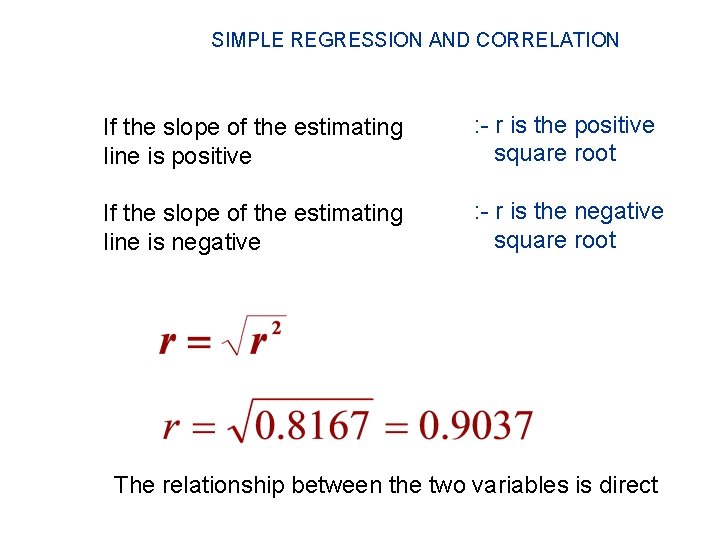
SIMPLE REGRESSION AND CORRELATION If the slope of the estimating line is positive : - r is the positive square root If the slope of the estimating line is negative : - r is the negative square root The relationship between the two variables is direct

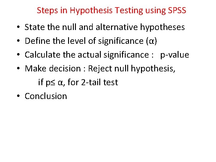
Steps in Hypothesis Testing using SPSS State the null and alternative hypotheses Define the level of significance (α) Calculate the actual significance : p-value Make decision : Reject null hypothesis, if p≤ α, for 2 -tail test • Conclusion • •

Scatter Plot Consider the example of the appliance store. The Data and Scatter Plot of the data: Scatter Plot 4. 5 Advertising Exp ($100 s) 1 2 3 4 5 Sales Rev ($1000 S) 1 1 2 2 4 4 3. 5 3 2. 5 Sales 2 1. 5 1 0. 5 0 0 1 2 3 4 5 6

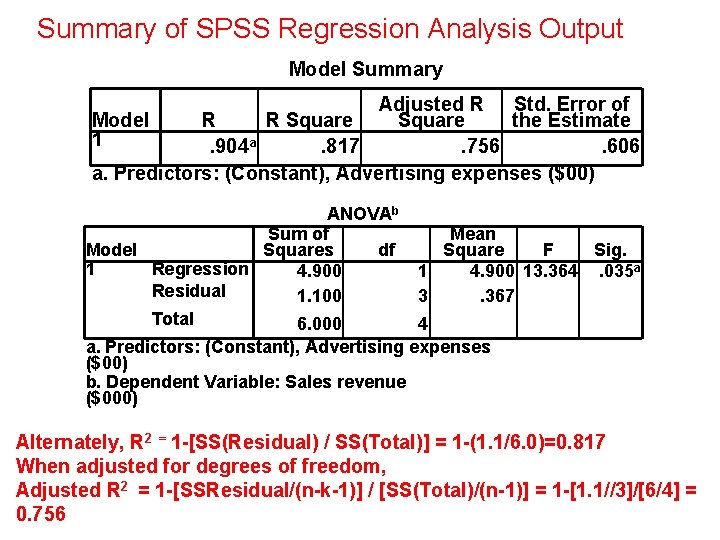
Summary of SPSS Regression Analysis Output Model Summary Adjusted R Std. Error of Model R R Square the Estimate 1. 904 a. 817. 756. 606 a. Predictors: (Constant), Advertising expenses ($00) ANOVAb Sum of Model Squares df 1 Regression 4. 900 Residual 1. 100 Total 6. 000 Mean Square F Sig. 1 4. 900 13. 364. 035 a 3. 367 4 a. Predictors: (Constant), Advertising expenses ($00) b. Dependent Variable: Sales revenue ($000) Alternately, R 2 = 1 -[SS(Residual) / SS(Total)] = 1 -(1. 1/6. 0)=0. 817 When adjusted for degrees of freedom, Adjusted R 2 = 1 -[SSResidual/(n-k-1)] / [SS(Total)/(n-1)] = 1 -[1. 1//3]/[6/4] = 0. 756

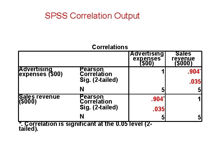
SPSS Correlation Output Correlations Advertising expenses ($00) Sales revenue ($000) Pearson Correlation Sig. (2 -tailed) N Pearson Correlation Sig. (2 -tailed) Advertising expenses ($00) 1 Sales revenue ($000). 904* 5. 904* . 035 5 1 . 035 5 5 N *. Correlation is significant at the 0. 05 level (2 tailed).

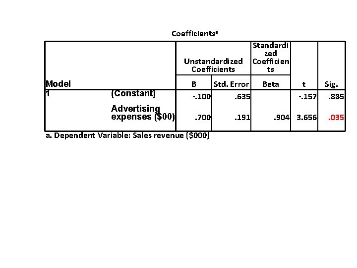
Coefficientsa Unstandardized Coefficients Model 1 (Constant) Advertising expenses ($00) B Std. Error -. 100. 635. 700 a. Dependent Variable: Sales revenue ($000) . 191 Standardi zed Coefficien ts Beta t Sig. -. 157. 885 . 904 3. 656 . 035

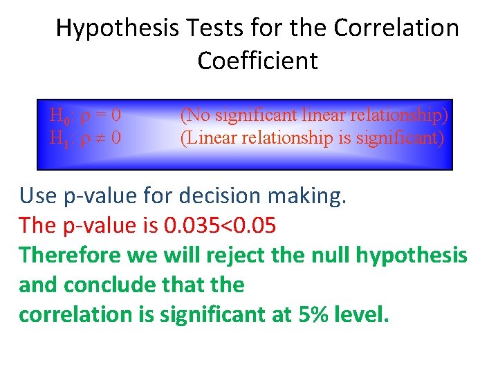
Hypothesis Tests for the Correlation Coefficient H 0: = 0 H 1: 0 (No significant linear relationship) (Linear relationship is significant) Use p-value for decision making. The p-value is 0. 035<0. 05 Therefore we will reject the null hypothesis and conclude that the correlation is significant at 5% level.

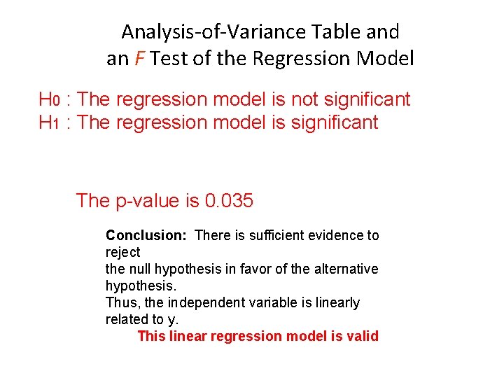
Analysis-of-Variance Table and an F Test of the Regression Model H 0 : The regression model is not significant H 1 : The regression model is significant The p-value is 0. 035 Conclusion: There is sufficient evidence to reject the null hypothesis in favor of the alternative hypothesis. Thus, the independent variable is linearly related to y. This linear regression model is valid

Testing for the existence of linear relationship n We test the hypothesis: H 0: b = 0 (the independent variable is not a significant predictor of the dependent variable) H 1: b is not equal to zero (the independent variable is a significant predictor of the dependent variable). n If b is not equal to zero (if the null hypothesis is rejected), we can conclude that the Independent variable contributes significantly in predicting the Dependent variable. Conclusion: The actual significance is 0. 035. Therefore we will reject the null hypothesis. The advertising expenses is a significant explanatory variable.

Multiple Regression Analysis Multiple regression uses many independent variables to predict or explain the variation in a dependent variables The basic multiple regression model is a first-order model, containing each predictor but no nonlinear terms such as squared values. In this model, each slope should be interpreted as a partial slope, the predicted effect of a onechange in a variable, holding all other variables constant.

Assumptions of the Multiple Linear Regression Model q The size of the sample has a direct impact on the statistical power of the significance testing in multiple regression. Power in multiple regression refers to the probability of detecting as statistically significant a specific level of R-square, or a regression coefficient at a specified significance level and a specific sample size. As a rule of thumb, there should be at least 20 times more cases than independent variables. q The measurement of the variables can be either continuous (metric) or dichotomous (non-metric). When the dependent variable is dichotomous (coded 0– 1), discriminant analysis is appropriate. q Linearity—As regression analysis is based on the concept of correlation, the linearity of the relationship between dependent and independent variables is important.

Assumptions of the Multiple Linear Regression Model q Homoscedasticity—The assumption of equal variances between pairs of variables. q Independence of Error Terms and Normality—It is assumed that errors of prediction (differences between the obtained and predicted dependent variable scores) are independent and normally distributed. q Multicollinearity— Multicollinearity denotes the situation where the independent/predictor variables are highly correlated. When independent variables are multicollinear, there is “overlap” or sharing of predictive power so that one variable can be highly explained or predicted by the other variable(s). Thus, that predictor variable adds little to the explanatory power of the entire set. Checking for Multicollinearity: In Multiple Regression using SPSS, it is possible to request the display of Tolerance and VIF values for each predictor as a check for multicollinearity. A tolerance value is an indication of the percent of variance in the predictor that cannot be accounted for by the other predictors. Hence, very small values indicate “overlap” or sharing of predictive power (i. e. , the predictor is redundant). Tolerance values that are less than 0. 10 may merit further investigation. The VIF, which stands for variance inflation factor, is computed as “ 1/tolerance, ” and it is suggested that predictor variables whose VIF values are greater than 10 may merit further investigation.

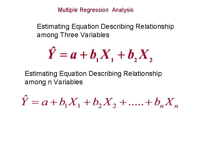
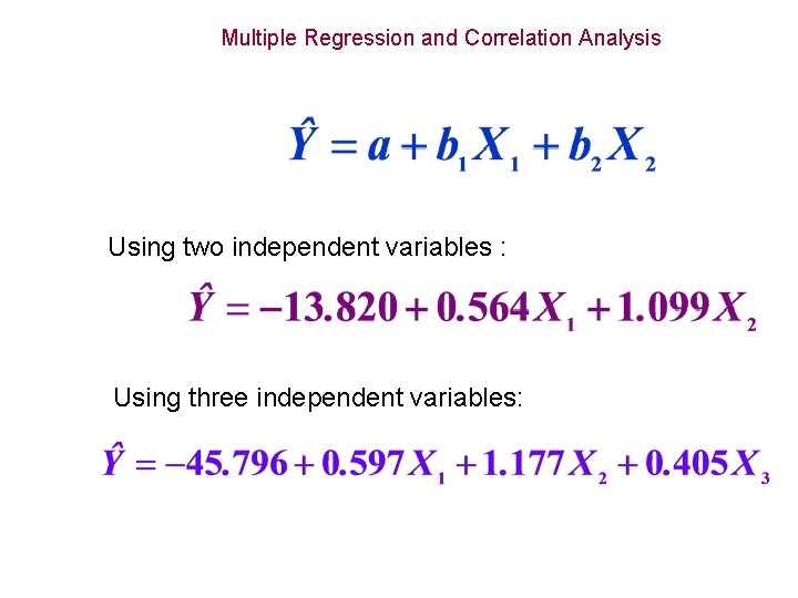
Multiple Regression Analysis Estimating Equation Describing Relationship among Three Variables Estimating Equation Describing Relationship among n Variables

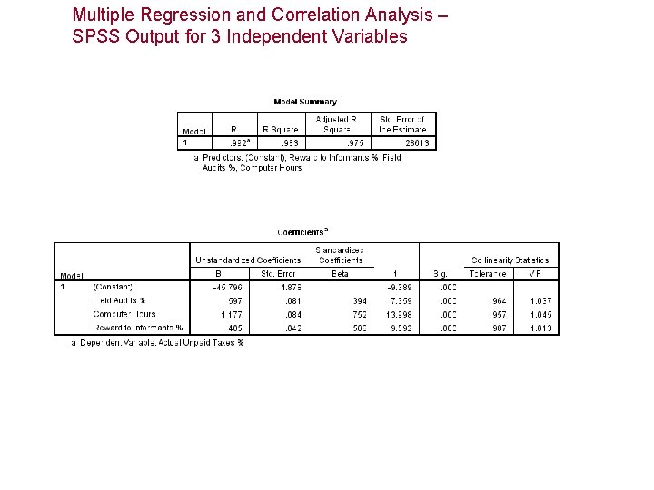
Multiple Regression Analysis – Example File: PPT_Mult. Regr The department is interested to know whether the amount of field audits and computer hours spent on tracking have yielded any results. Further the department has introduced the reward system for tracking the culprits. The data on actual unpaid taxes for ten cases is considered for analysis. Initially the regression of Actual Unpaid Taxes(Y) on Field Audits(X 1) and Computer Hours(X 2) was carried out and as a next step the Reward to Informants(X 3) was also considered as a variable and analyzed. The analysis yielded the following SPSS outputs.

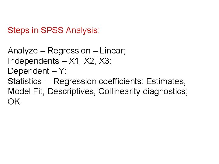
Steps in SPSS Analysis: Analyze – Regression – Linear; Independents – X 1, X 2, X 3; Dependent – Y; Statistics – Regression coefficients: Estimates, Model Fit, Descriptives, Collinearity diagnostics; OK

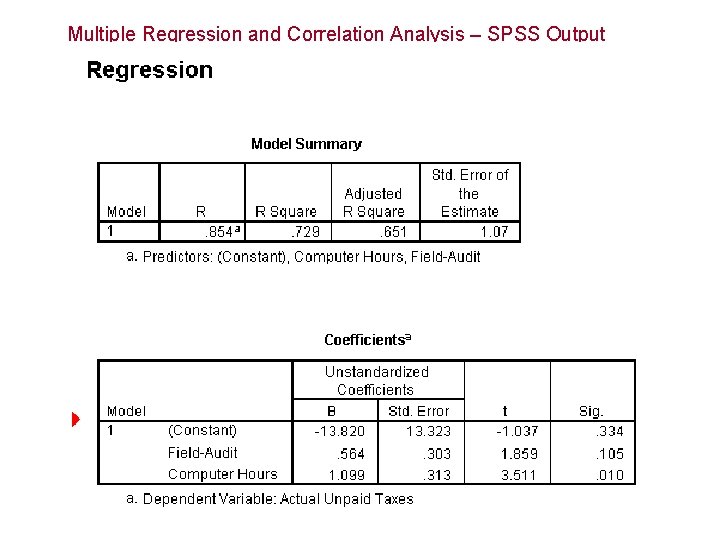
Multiple Regression and Correlation Analysis – SPSS Output

Multiple Regression and Correlation Analysis – SPSS Output for 3 Independent Variables

Multiple Regression and Correlation Analysis Using two independent variables : Using three independent variables:

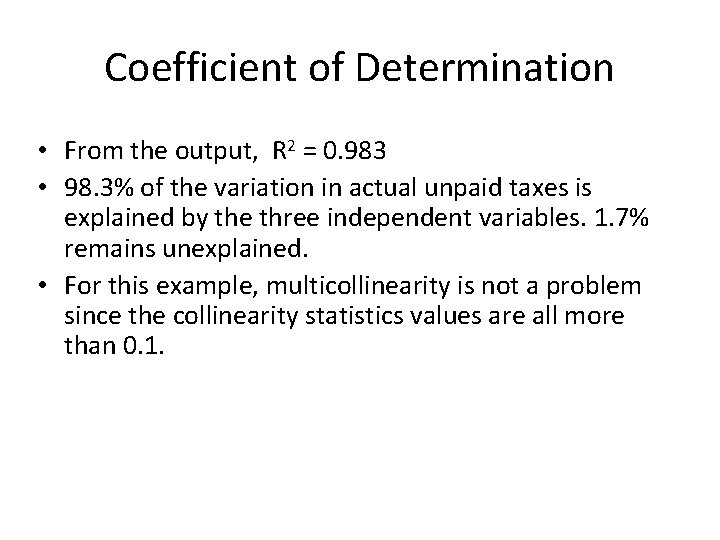
Coefficient of Determination • From the output, R 2 = 0. 983 • 98. 3% of the variation in actual unpaid taxes is explained by the three independent variables. 1. 7% remains unexplained. • For this example, multicollinearity is not a problem since the collinearity statistics values are all more than 0. 1.

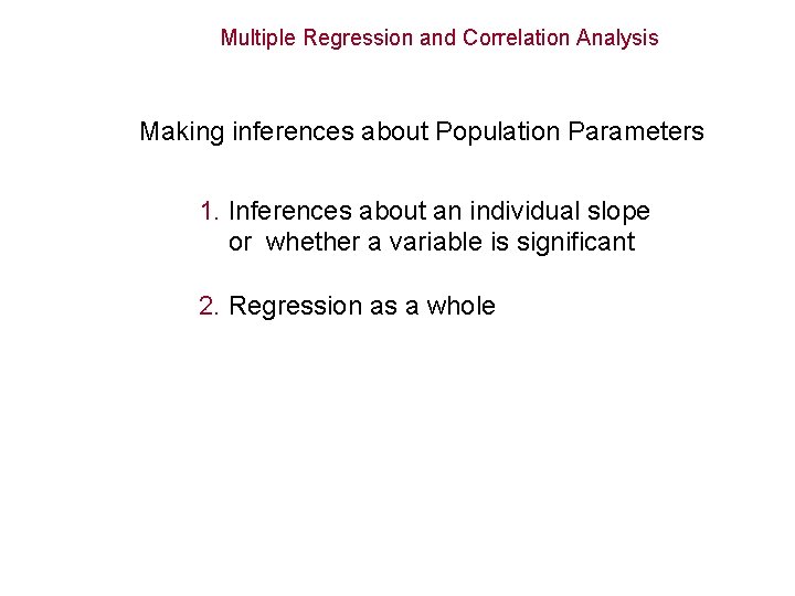
Multiple Regression and Correlation Analysis Making inferences about Population Parameters 1. Inferences about an individual slope or whether a variable is significant 2. Regression as a whole

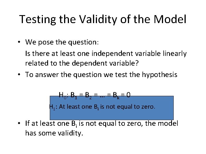
Testing the Validity of the Model • We pose the question: Is there at least one independent variable linearly related to the dependent variable? • To answer the question we test the hypothesis H 0 : B 1 = B 2 = … = B k = 0 H 1: At least one Bi is not equal to zero. • If at least one Bi is not equal to zero, the model has some validity.

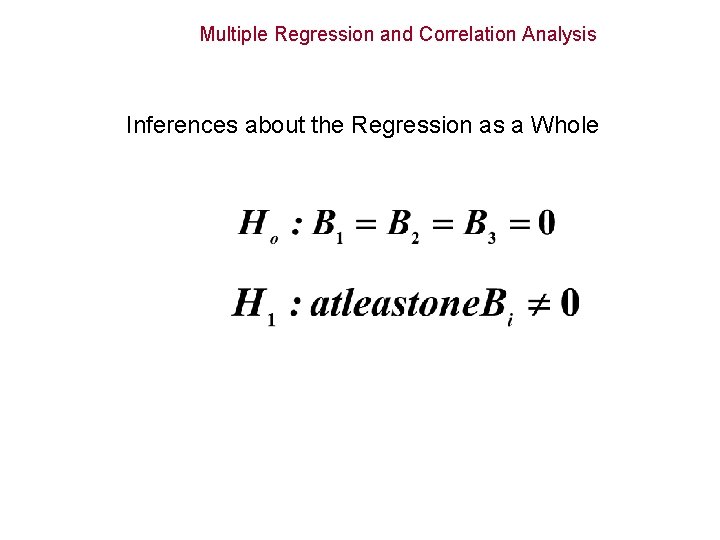
Multiple Regression and Correlation Analysis Inferences about the Regression as a Whole

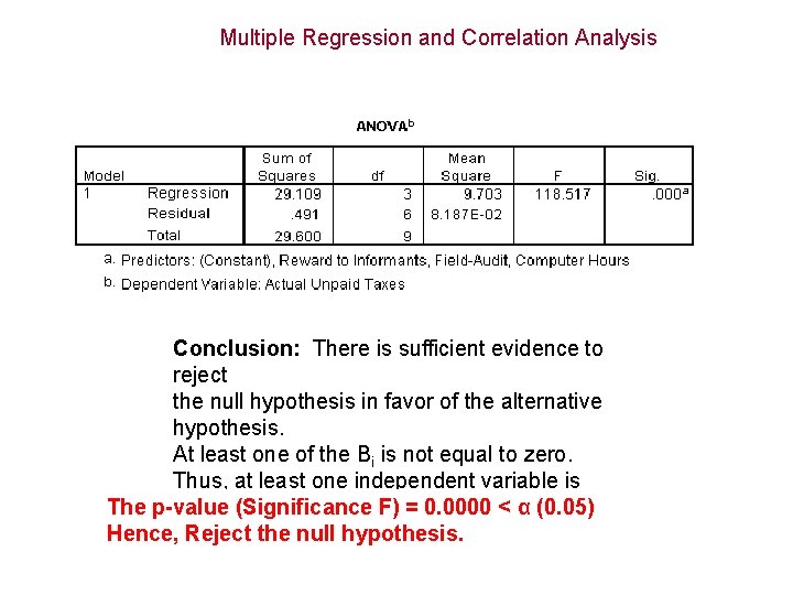
Multiple Regression and Correlation Analysis Conclusion: There is sufficient evidence to reject the null hypothesis in favor of the alternative hypothesis. At least one of the Bi is not equal to zero. Thus, at least one independent variable is The p-value linearly(Significance related to y. F) = 0. 0000 < α (0. 05) Hence, Reject null regression hypothesis. model is valid Thisthe linear

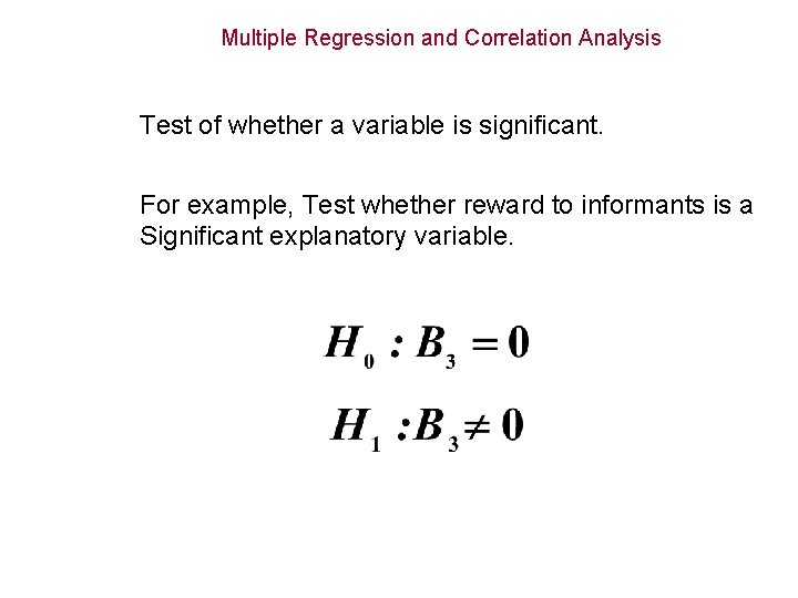
Multiple Regression and Correlation Analysis Test of whether a variable is significant. For example, Test whether reward to informants is a Significant explanatory variable.

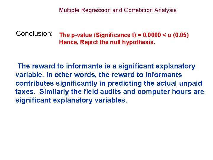
Multiple Regression and Correlation Analysis Conclusion: The p-value (Significance t) = 0. 0000 < α (0. 05) Hence, Reject the null hypothesis. The reward to informants is a significant explanatory variable. In other words, the reward to informants contributes significantly in predicting the actual unpaid taxes. Similarly the field audits and computer hours are significant explanatory variables.

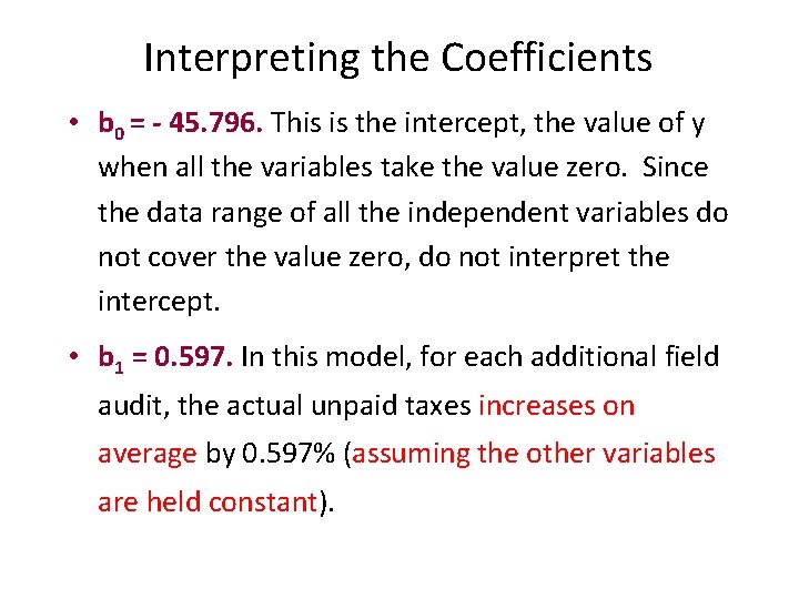
Interpreting the Coefficients • b 0 = - 45. 796. This is the intercept, the value of y when all the variables take the value zero. Since the data range of all the independent variables do not cover the value zero, do not interpret the intercept. • b 1 = 0. 597. In this model, for each additional field audit, the actual unpaid taxes increases on average by 0. 597% (assuming the other variables are held constant).

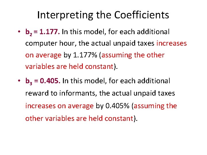
Interpreting the Coefficients • b 2 = 1. 177. In this model, for each additional computer hour, the actual unpaid taxes increases on average by 1. 177% (assuming the other variables are held constant). • b 3 = 0. 405. In this model, for each additional reward to informants, the actual unpaid taxes increases on average by 0. 405% (assuming the other variables are held constant).

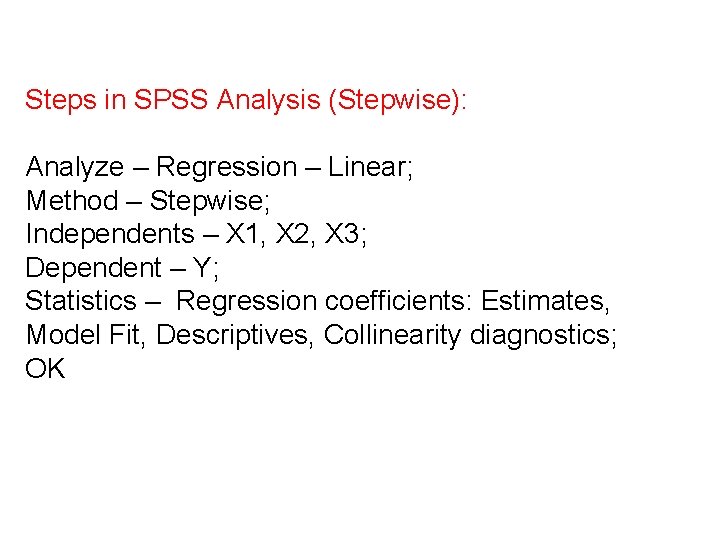
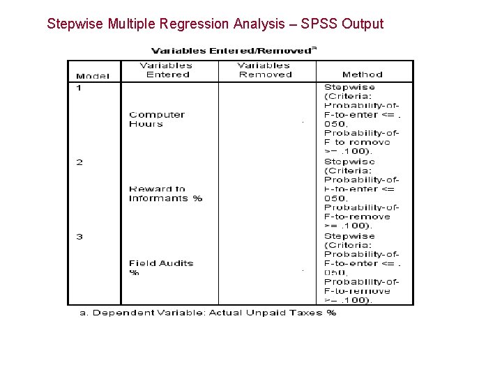
Steps in SPSS Analysis (Stepwise): Analyze – Regression – Linear; Method – Stepwise; Independents – X 1, X 2, X 3; Dependent – Y; Statistics – Regression coefficients: Estimates, Model Fit, Descriptives, Collinearity diagnostics; OK

Stepwise Multiple Regression Analysis – SPSS Output

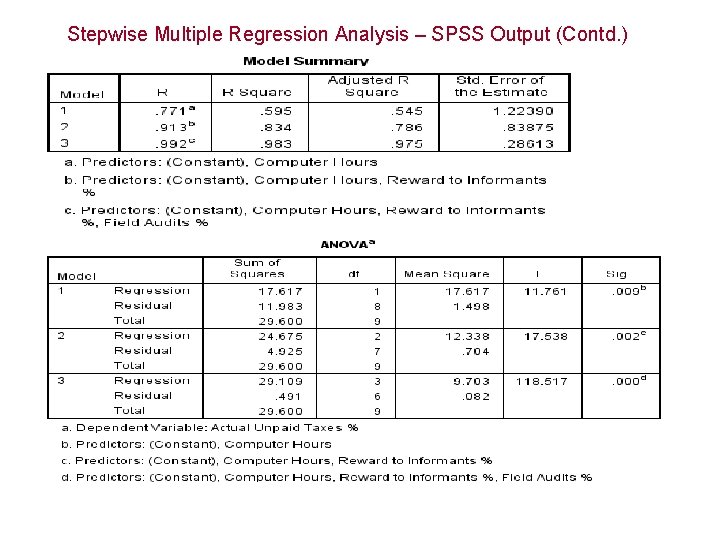
Stepwise Multiple Regression Analysis – SPSS Output (Contd. )

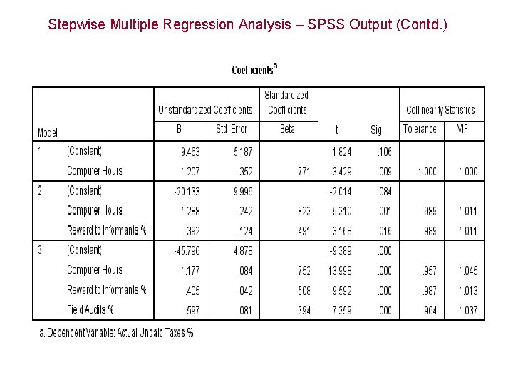
Stepwise Multiple Regression Analysis – SPSS Output (Contd. )

Coefficient of Determination • From the output, • R 2 = 0. 595 for Model 1. That means 59. 5% of the variation in actual unpaid taxes is explained by the most significant independent variable computer hours. • R 2 = 0. 834 for Model 2. That means 83. 4% of the variation in actual unpaid taxes is explained by the two independent variables computer hours and reward to informants. The incremental explanation attributed to the variable reward to informants is 23. 9%. • R 2 = 0. 983 for Model 3. That means 98. 3% of the variation in actual unpaid taxes is explained by the three independent variables. 1. 7% remains unexplained. • For this example, multicollinearity is not a problem since the collinearity statistics values are all more than 0. 1.