Moderated Multiple Regression Class 18 Functions of Regression

Moderated Multiple Regression Class 18

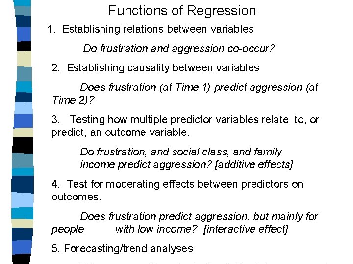
Functions of Regression 1. Establishing relations between variables Do frustration and aggression co-occur? 2. Establishing causality between variables Does frustration (at Time 1) predict aggression (at Time 2)? 3. Testing how multiple predictor variables relate to, or predict, an outcome variable. Do frustration, and social class, and family income predict aggression? [additive effects] 4. Test for moderating effects between predictors on outcomes. Does frustration predict aggression, but mainly for people with low income? [interactive effect] 5. Forecasting/trend analyses

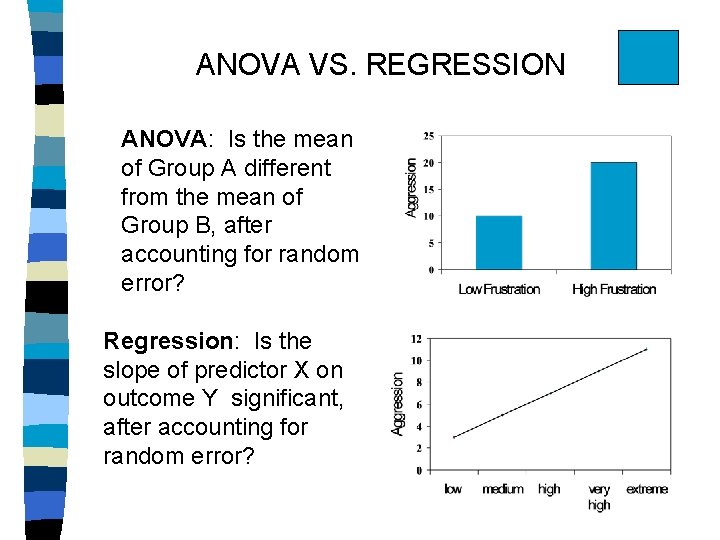
ANOVA VS. REGRESSION ANOVA: Is the mean of Group A different from the mean of Group B, after accounting for random error? Regression: Is the slope of predictor X on outcome Y significant, after accounting for random error?

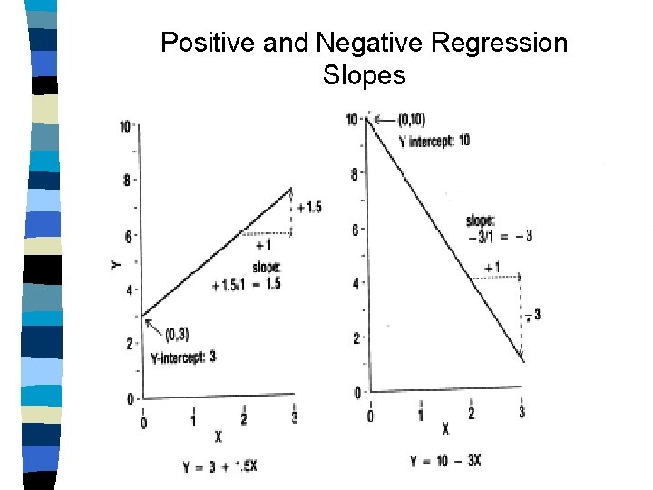
Positive and Negative Regression Slopes

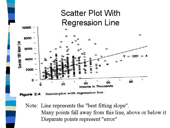
Scatter Plot With Regression Line Note: Line represents the "best fitting slope". Many points fall away from this line, above or below it Disparate points represent "error"

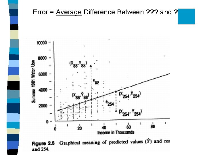
Error = Average Difference Between ? ? ? and ? ? ?

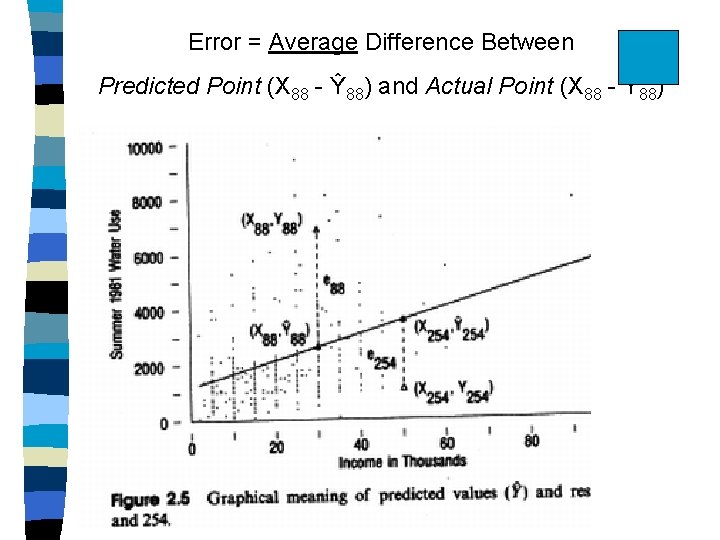
Error = Average Difference Between Predicted Point (X 88 - Ŷ 88) and Actual Point (X 88 - Y 88)

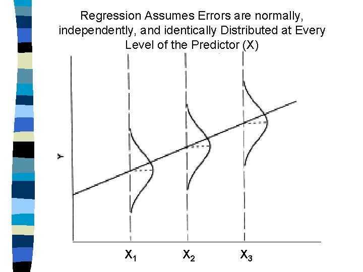
Regression Assumes Errors are normally, independently, and identically Distributed at Every Level of the Predictor (X) X 1 X 2 X 3

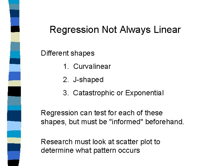
Regression Not Always Linear Different shapes 1. Curvalinear 2. J-shaped 3. Catastrophic or Exponential Regression can test for each of these shapes, but must be "informed" beforehand. Research must look at scatter plot to determine what pattern occurs

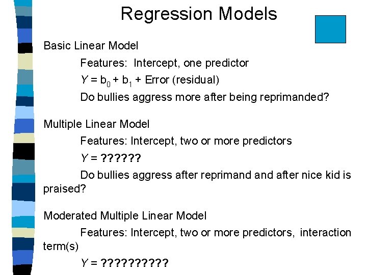
Regression Models Basic Linear Model Features: Intercept, one predictor Y = b 0 + b 1 + Error (residual) Do bullies aggress more after being reprimanded? Multiple Linear Model Features: Intercept, two or more predictors Y = ? ? ? Do bullies aggress after reprimand after nice kid is praised? Moderated Multiple Linear Model Features: Intercept, two or more predictors, interaction term(s) Y = ? ? ? ? ?

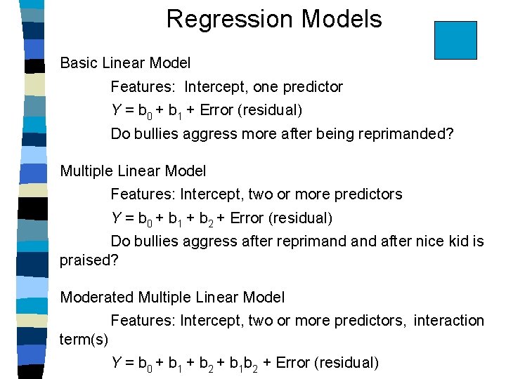
Regression Models Basic Linear Model Features: Intercept, one predictor Y = b 0 + b 1 + Error (residual) Do bullies aggress more after being reprimanded? Multiple Linear Model Features: Intercept, two or more predictors Y = b 0 + b 1 + b 2 + Error (residual) Do bullies aggress after reprimand after nice kid is praised? Moderated Multiple Linear Model Features: Intercept, two or more predictors, interaction term(s) Y = b 0 + b 1 + b 2 + b 1 b 2 + Error (residual)

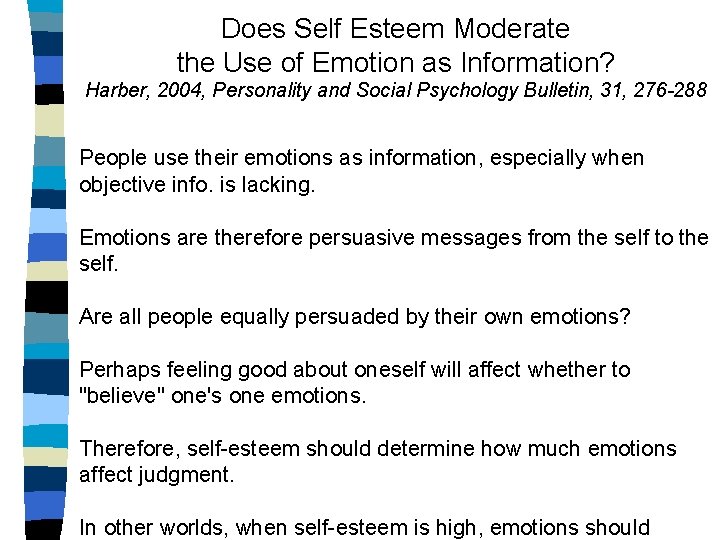
Does Self Esteem Moderate the Use of Emotion as Information? Harber, 2004, Personality and Social Psychology Bulletin, 31, 276 -288 People use their emotions as information, especially when objective info. is lacking. Emotions are therefore persuasive messages from the self to the self. Are all people equally persuaded by their own emotions? Perhaps feeling good about oneself will affect whether to "believe" one's one emotions. Therefore, self-esteem should determine how much emotions affect judgment. In other worlds, when self-esteem is high, emotions should

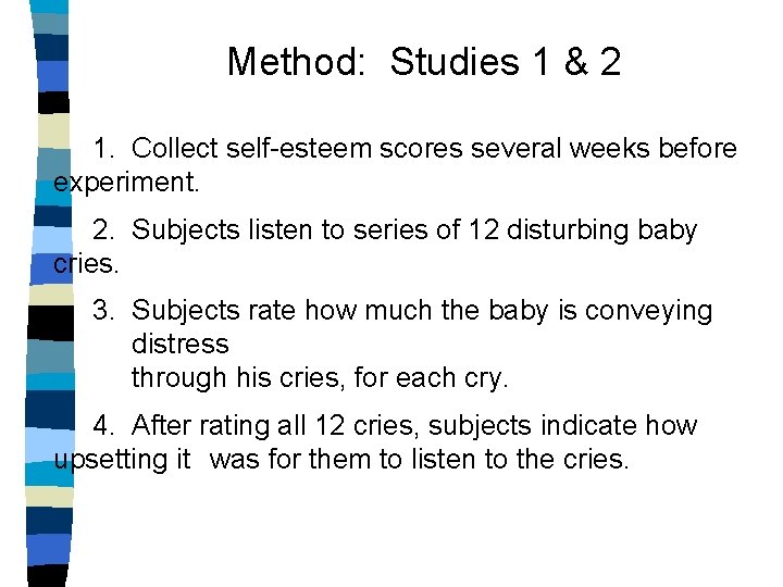
Method: Studies 1 & 2 1. Collect self-esteem scores several weeks before experiment. 2. Subjects listen to series of 12 disturbing baby cries. 3. Subjects rate how much the baby is conveying distress through his cries, for each cry. 4. After rating all 12 cries, subjects indicate how upsetting it was for them to listen to the cries.

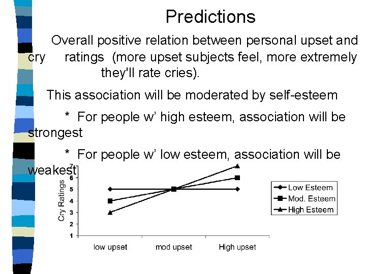
Predictions Overall positive relation between personal upset and cry ratings (more upset subjects feel, more extremely they'll rate cries). This association will be moderated by self-esteem * For people w’ high esteem, association will be strongest * For people w’ low esteem, association will be weakest.

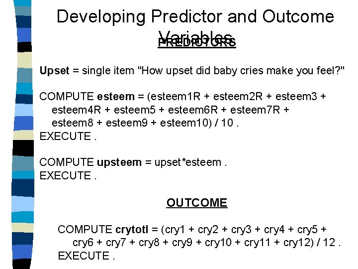
Developing Predictor and Outcome Variables PREDICTORS Upset = single item "How upset did baby cries make you feel? " COMPUTE esteem = (esteem 1 R + esteem 2 R + esteem 3 + esteem 4 R + esteem 5 + esteem 6 R + esteem 7 R + esteem 8 + esteem 9 + esteem 10) / 10. EXECUTE. COMPUTE upsteem = upset*esteem. EXECUTE. OUTCOME COMPUTE crytotl = (cry 1 + cry 2 + cry 3 + cry 4 + cry 5 + cry 6 + cry 7 + cry 8 + cry 9 + cry 10 + cry 11 + cry 12) / 12. EXECUTE.

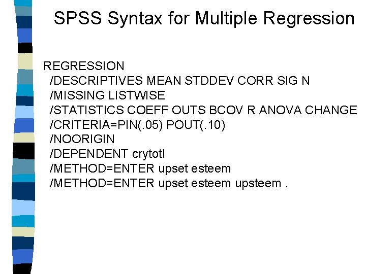
SPSS Syntax for Multiple Regression REGRESSION /DESCRIPTIVES MEAN STDDEV CORR SIG N /MISSING LISTWISE /STATISTICS COEFF OUTS BCOV R ANOVA CHANGE /CRITERIA=PIN(. 05) POUT(. 10) /NOORIGIN /DEPENDENT crytotl /METHOD=ENTER upset esteem upsteem.

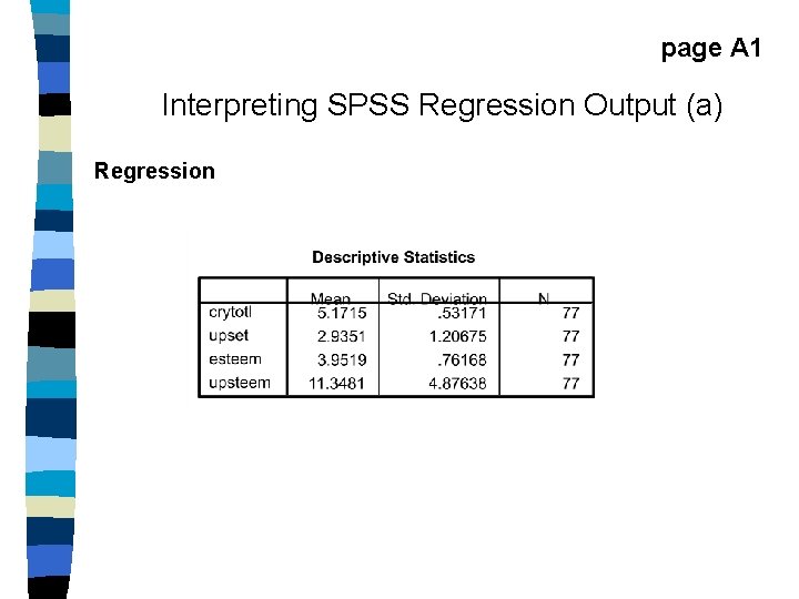
page A 1 Interpreting SPSS Regression Output (a) Regression

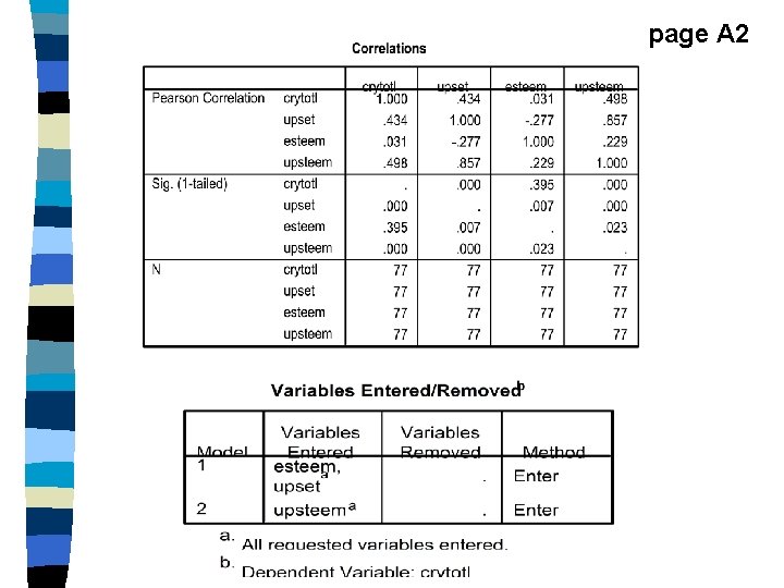
page A 2

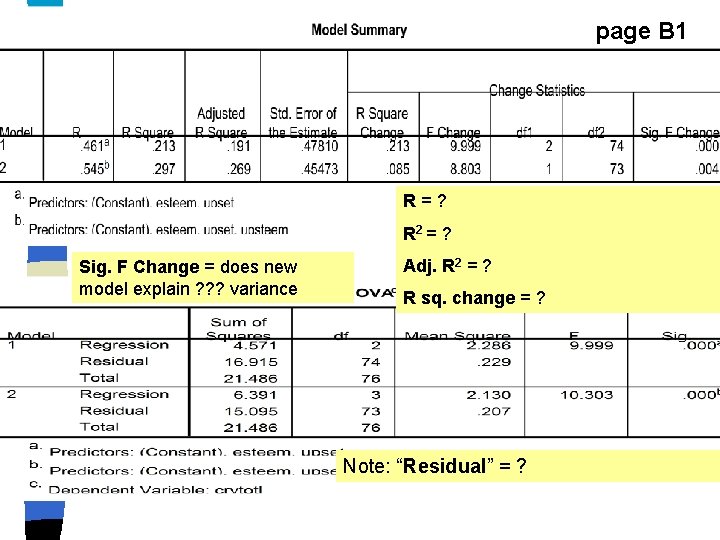
page B 1 R=? R 2 = ? Sig. F Change = does new model explain ? ? ? variance Adj. R 2 = ? R sq. change = ? Note: “Residual” = ?

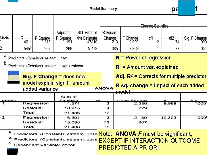
page B 1 R = Power of regression R 2 = Amount var. explained Sig. F Change = does new model explain signif. amount added variance Adj. R 2 = Corrects for multiple predictors R sq. change = Impact of each added model Note: ANOVA F must be significant, EXCEPT IF INTERACTION OUTCOME PREDICTED A-PRIORI

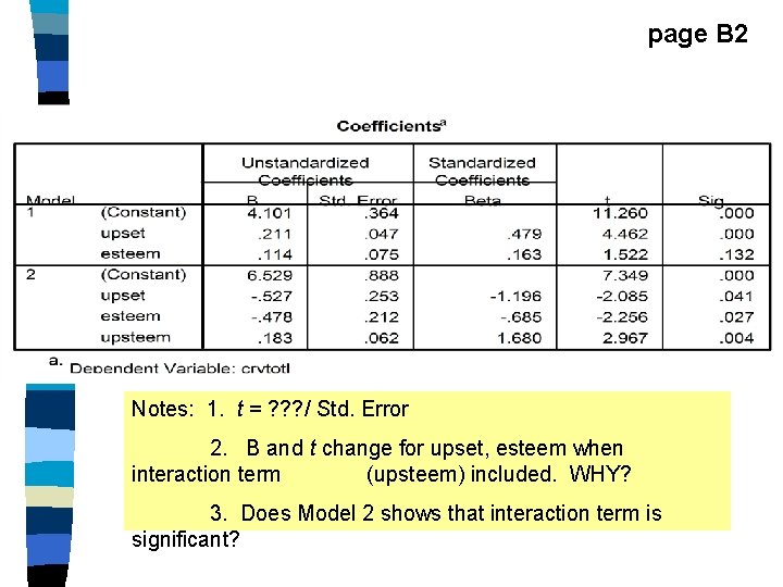
page B 2 Notes: 1. t = ? ? ? / Std. Error 2. B and t change for upset, esteem when interaction term (upsteem) included. WHY? 3. Does Model 2 shows that interaction term is significant?

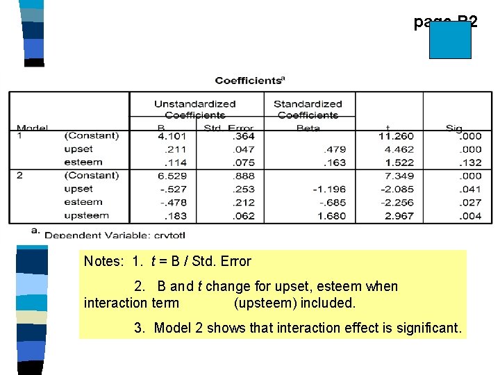
page B 2 Notes: 1. t = B / Std. Error 2. B and t change for upset, esteem when interaction term (upsteem) included. 3. Model 2 shows that interaction effect is significant.

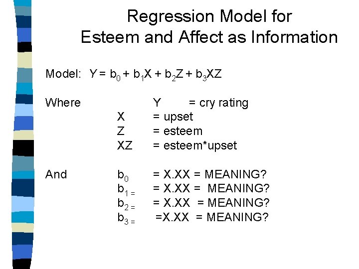
Regression Model for Esteem and Affect as Information Model: Y = b 0 + b 1 X + b 2 Z + b 3 XZ Where And X Z XZ Y = cry rating = upset = esteem*upset b 0 b 1 = b 2 = b 3 = = X. XX = MEANING? =X. XX = MEANING?

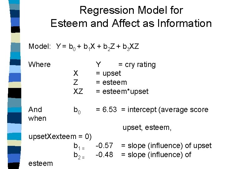
Regression Model for Esteem and Affect as Information Model: Y = b 0 + b 1 X + b 2 Z + b 3 XZ Where And when X Z XZ Y = cry rating = upset = esteem*upset b 0 = 6. 53 = intercept (average score upset, esteem, upset. Xexteem = 0) b 1 = -0. 57 b 2 = -0. 48 esteem = slope (influence) of upset = slope (influence) of

Plotting Outcome: Baby Cry Ratings as a Function of Listener's Upset and Listener's Self Esteem ? ? ?

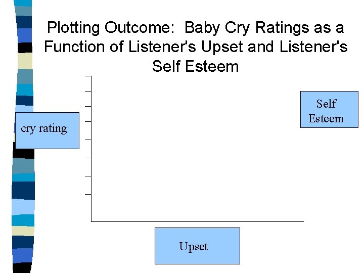
Plotting Outcome: Baby Cry Ratings as a Function of Listener's Upset and Listener's Self Esteem cry rating Upset

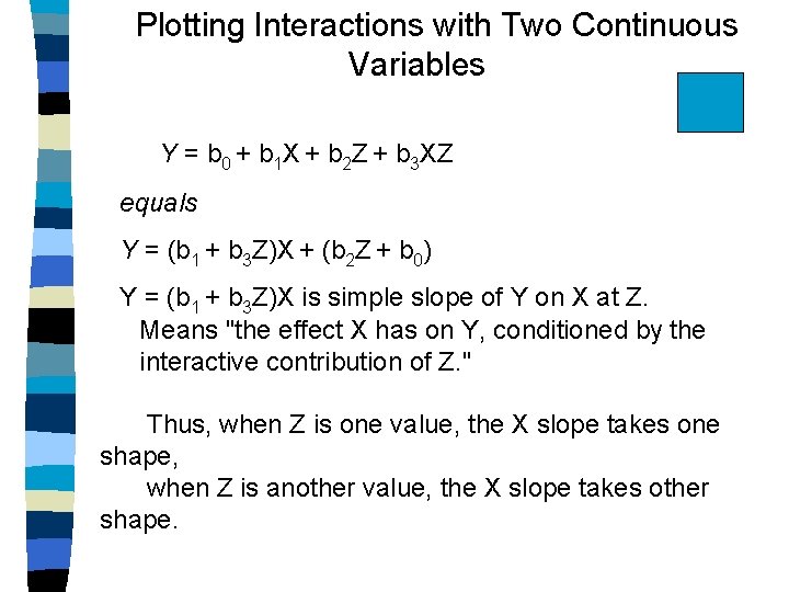
Plotting Interactions with Two Continuous Variables Y = b 0 + b 1 X + b 2 Z + b 3 XZ equals Y = (b 1 + b 3 Z)X + (b 2 Z + b 0) Y = (b 1 + b 3 Z)X is simple slope of Y on X at Z. Means "the effect X has on Y, conditioned by the interactive contribution of Z. " Thus, when Z is one value, the X slope takes one shape, when Z is another value, the X slope takes other shape.

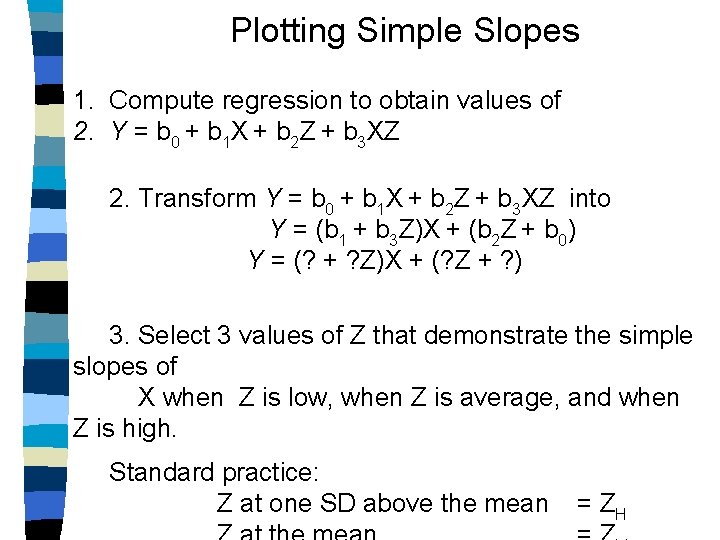
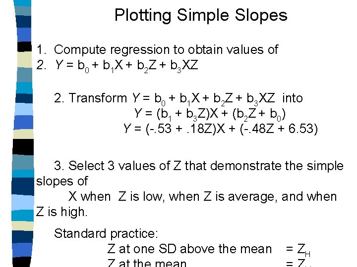
Plotting Simple Slopes 1. Compute regression to obtain values of 2. Y = b 0 + b 1 X + b 2 Z + b 3 XZ 2. Transform Y = b 0 + b 1 X + b 2 Z + b 3 XZ into Y = (b 1 + b 3 Z)X + (b 2 Z + b 0) Y = (? + ? Z)X + (? Z + ? ) 3. Select 3 values of Z that demonstrate the simple slopes of X when Z is low, when Z is average, and when Z is high. Standard practice: Z at one SD above the mean = ZH

Plotting Simple Slopes 1. Compute regression to obtain values of 2. Y = b 0 + b 1 X + b 2 Z + b 3 XZ 2. Transform Y = b 0 + b 1 X + b 2 Z + b 3 XZ into Y = (b 1 + b 3 Z)X + (b 2 Z + b 0) Y = (-. 53 +. 18 Z)X + (-. 48 Z + 6. 53) 3. Select 3 values of Z that demonstrate the simple slopes of X when Z is low, when Z is average, and when Z is high. Standard practice: Z at one SD above the mean = ZH

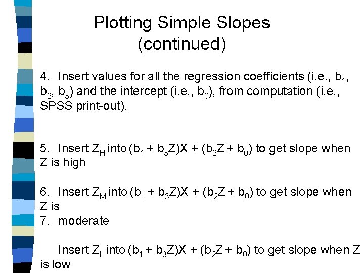
Plotting Simple Slopes (continued) 4. Insert values for all the regression coefficients (i. e. , b 1, b 2, b 3) and the intercept (i. e. , b 0), from computation (i. e. , SPSS print-out). 5. Insert ZH into (b 1 + b 3 Z)X + (b 2 Z + b 0) to get slope when Z is high 6. Insert ZM into (b 1 + b 3 Z)X + (b 2 Z + b 0) to get slope when Z is 7. moderate Insert ZL into (b 1 + b 3 Z)X + (b 2 Z + b 0) to get slope when Z is low

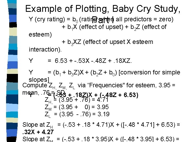
Example of Plotting, Baby Cry Study, Y (cry rating) = b 0 (rating when. I all predictors = zero) Part esteem) + b 1 X (effect of upset) + b 2 Z (effect of + b 3 XZ (effect of upset X esteem interaction). Y = 6. 53 + -. 53 X -. 48 Z +. 18 XZ. Y = (b 1 + b 3 Z)X + (b 2 Z + b 0) [conversion for simple slopes] Compute ZH, ZM, ZL via “Frequencies" for esteem, 3. 95 = mean, SD +. 18 Z)X + (-. 48 Z + 6. 53) Y. 76==(-. 53 ZH, = (3. 95 +. 76) = 4. 71 ZM = (3. 95 + 0) = 3. 95 ZL = (3. 95 -. 76) = 3. 19 Slope at ZH = (-. 53 +. 18 * 4. 71)X + ([-. 48 * 4. 71] + 6. 53) =. 32 X + 4. 27 Slope at Z = (-. 53 +. 18 * 3. 95)X + ([-. 48 * 3. 95] + 6. 53) =

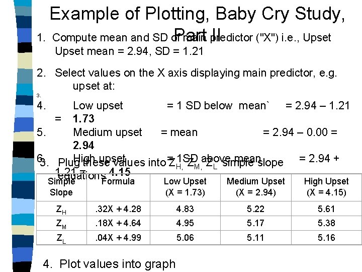
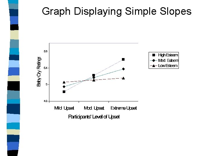
Example of Plotting, Baby Cry Study, Part II 1. Compute mean and SD of main predictor ("X") i. e. , Upset mean = 2. 94, SD = 1. 21 2. Select values on the X axis displaying main predictor, e. g. upset at: 3. 4. Low upset = 1 SD below mean` = 2. 94 – 1. 21 = 1. 73 5. Medium upset = mean = 2. 94 – 0. 00 = 2. 94 6. High upset 1 SD meanslope = 2. 94 + 3. Plug these values into =ZH, ZM, above ZL simple 1. 21 = 4. 15 equations Simple Slope Formula Low Upset (X = 1. 73) Medium Upset (X = 2. 94) High Upset (X = 4. 15) ZH . 32 X + 4. 28 4. 83 5. 22 5. 61 ZM . 18 X + 4. 64 4. 95 5. 17 5. 38 ZL . 04 X + 4. 99 5. 06 5. 11 5. 16 4. Plot values into graph

Graph Displaying Simple Slopes

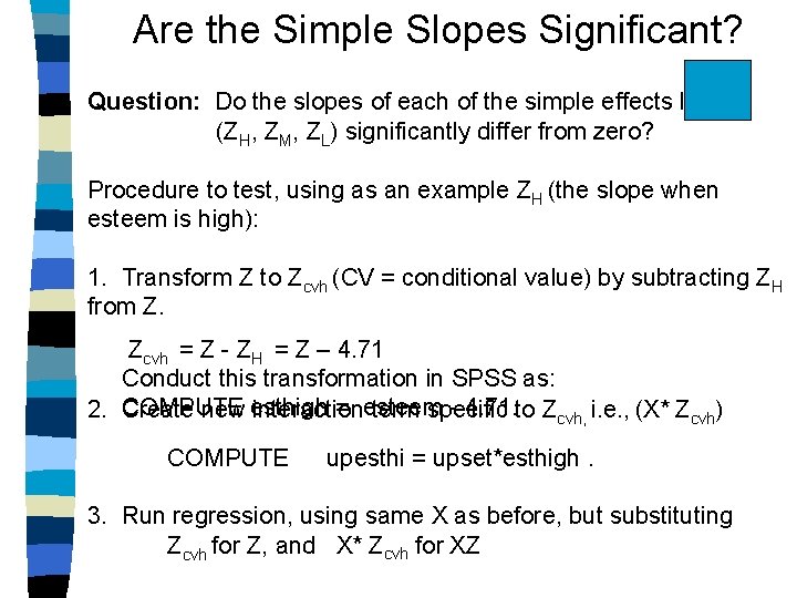
Are the Simple Slopes Significant? Question: Do the slopes of each of the simple effects lines (ZH, ZM, ZL) significantly differ from zero? Procedure to test, using as an example ZH (the slope when esteem is high): 1. Transform Z to Zcvh (CV = conditional value) by subtracting ZH from Z. Zcvh = Z - ZH = Z – 4. 71 Conduct this transformation in SPSS as: = esteem - 4. 71. to Zcvh, i. e. , (X* Zcvh) 2. COMPUTE Create new esthigh interaction term specific COMPUTE upesthi = upset*esthigh. 3. Run regression, using same X as before, but substituting Zcvh for Z, and X* Zcvh for XZ

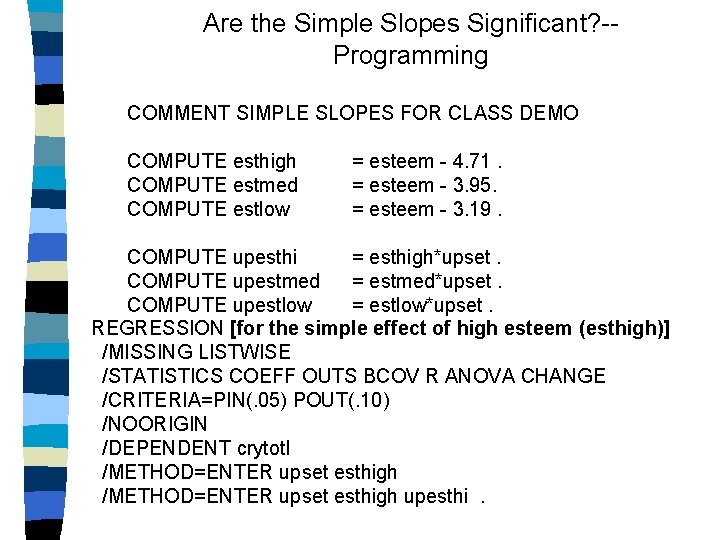
Are the Simple Slopes Significant? -Programming COMMENT SIMPLE SLOPES FOR CLASS DEMO COMPUTE esthigh COMPUTE estmed COMPUTE estlow = esteem - 4. 71. = esteem - 3. 95. = esteem - 3. 19. COMPUTE upesthi = esthigh*upset. COMPUTE upestmed = estmed*upset. COMPUTE upestlow = estlow*upset. REGRESSION [for the simple effect of high esteem (esthigh)] /MISSING LISTWISE /STATISTICS COEFF OUTS BCOV R ANOVA CHANGE /CRITERIA=PIN(. 05) POUT(. 10) /NOORIGIN /DEPENDENT crytotl /METHOD=ENTER upset esthigh upesthi.

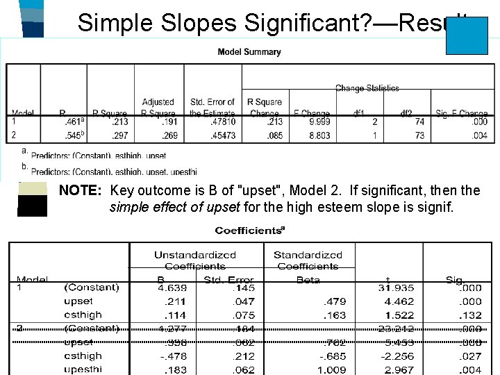
Simple Slopes Significant? —Results Regression NOTE: Key outcome is B of "upset", Model 2. If significant, then the simple effect of upset for the high esteem slope is signif.

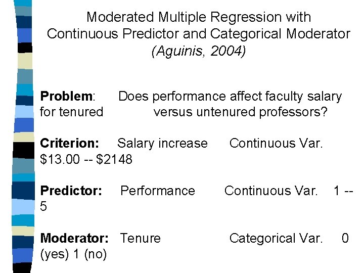
Moderated Multiple Regression with Continuous Predictor and Categorical Moderator (Aguinis, 2004) Problem: for tenured Does performance affect faculty salary versus untenured professors? Criterion: Salary increase $13. 00 -- $2148 Predictor: 5 Performance Moderator: Tenure (yes) 1 (no) Continuous Var. Categorical Var. 1 -0

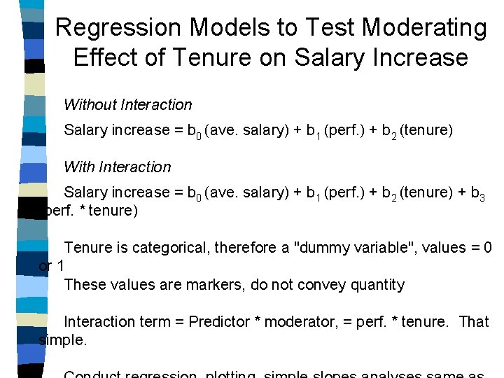
Regression Models to Test Moderating Effect of Tenure on Salary Increase Without Interaction Salary increase = b 0 (ave. salary) + b 1 (perf. ) + b 2 (tenure) With Interaction Salary increase = b 0 (ave. salary) + b 1 (perf. ) + b 2 (tenure) + b 3 (perf. * tenure) Tenure is categorical, therefore a "dummy variable", values = 0 or 1 These values are markers, do not convey quantity Interaction term = Predictor * moderator, = perf. * tenure. That simple.

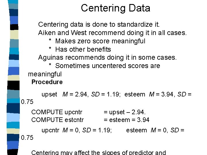
Centering Data Centering data is done to standardize it. Aiken and West recommend doing it in all cases. * Makes zero score meaningful * Has other benefits Aguinas recommends doing it in some cases. * Sometimes uncentered scores are meaningful Procedure upset M = 2. 94, SD = 1. 19; esteem M = 3. 94, SD = 0. 75 COMPUTE upcntr COMPUTE estcntr = upset – 2. 94. = esteem = 3. 94 upcntr M = 0, SD = 1. 19; esteem M = 0, SD = 0. 75 Centering may affect the slopes of predictor and

THE KENT AND HERMAN DIALOGUE A Moderated Multiple Regression Drama With A Satisfactory Conclusion Appropriate for All Audiences

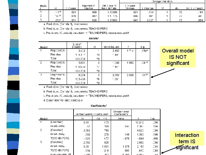
Overall model IS NOT significant Interaction term IS significant

Act 1, Scene 1: Kent contacts Herman regarding this vexing conundrum. Dear Dr. Aguinis, I am using your text in my graduate methods course. It is very clear and straightforward, which both my students and I appreciate. A question came up that I thought you might be able to answer. If an MMR model produces a significant interaction, but the ANOVA F is not itself significant, is the significant interaction still a valid result? My impression is that the F of the overall model (as indicated by the ANOVA F and/or by the R-sqr. change) must be significant. Thank you for your response, Kent Harber

Act 1, scene 2: Herman replies! Kent, I believe you are referring to a test of a targeted interaction effect without looking at the overall (omnibus) effect. Please see pp. 134 -135 of the book. Let me know if this does not answer your question and I will be delighted to follow up with you. Thanks for your kind words about my book! All the best, --Herman.

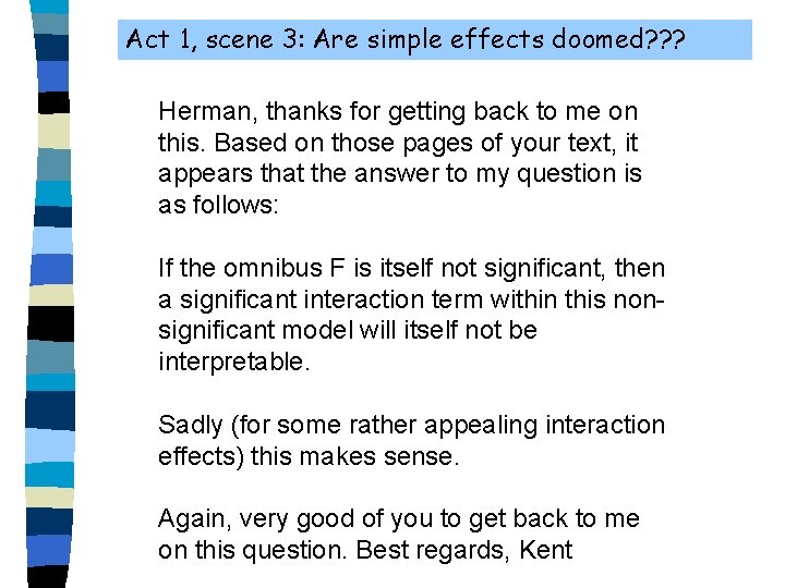
Act 1, scene 3: Are simple effects doomed? ? ? Herman, thanks for getting back to me on this. Based on those pages of your text, it appears that the answer to my question is as follows: If the omnibus F is itself not significant, then a significant interaction term within this nonsignificant model will itself not be interpretable. Sadly (for some rather appealing interaction effects) this makes sense. Again, very good of you to get back to me on this question. Best regards, Kent

Act 1, scene 4: Herman sustains the dramatic tension. Kent, Before I give you an answer and to make sure I understand the question. What do you mean precisely by "the ANOVA F test"? Regards, --Herman.

Act 1, scene 4: Herman drops the Big Clue Kent, Thanks for the clarification. Now, I understand your question perfectly. An article by Bedeian and Mossholder (1994), J. of Management, addresses this question directly. The full citation is on page 177 of my book. All the best, --Herman.

Finale: Simple effects are redeemed!!! [enter marching band, stage right]

Data Management Issues Setting up data file Checking accuracy of data Disposition of data Why obsess on these details? Murphy's Law If something can go wrong, it will go wrong, and at the worst possible time.

Creating a Coding Master 1. Get survey copy 2. Assign variable names 3. Assign variable values 4. Assign missing values 5. Proof master for accuracy 6. Make spare copy, keep in file drawer

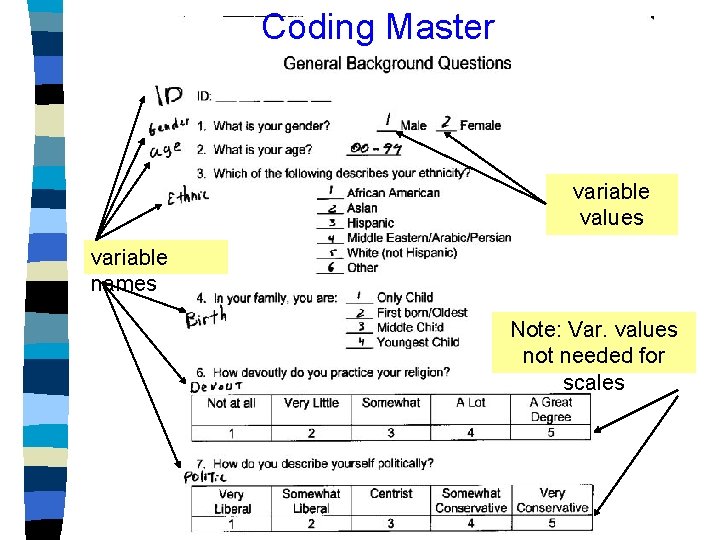
Coding Master variable values variable names Note: Var. values not needed for scales

Cleaning Data Set 1. Exercise in delay of gratification 2. Purpose: Reduce random error 3. Improve power of inferential stats.

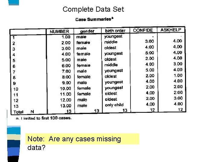
Complete Data Set Note: Are any cases missing data?

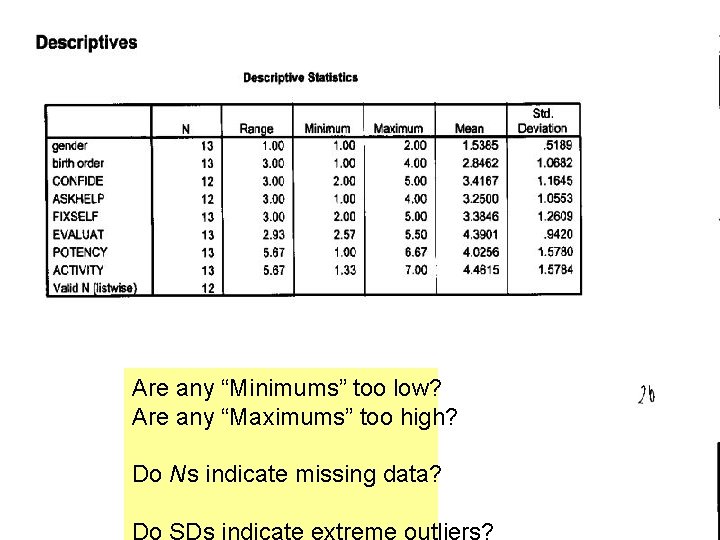
Are any “Minimums” too low? Are any “Maximums” too high? Do Ns indicate missing data? Do SDs indicate extreme outliers?

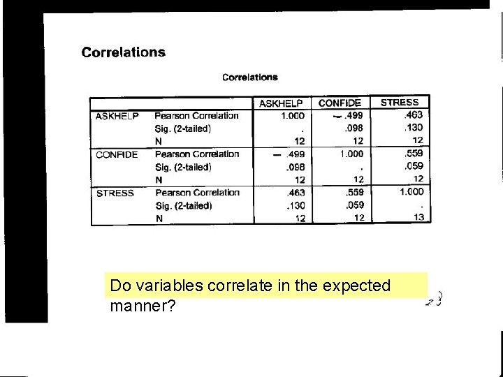
Do variables correlate in the expected manner?

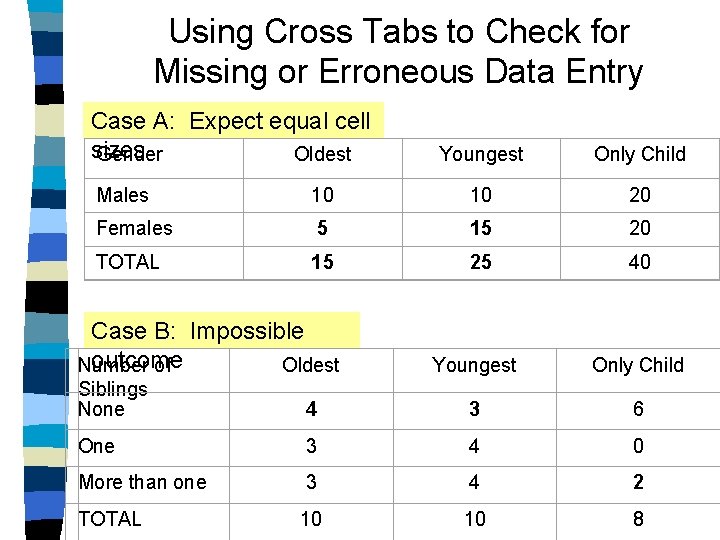
Using Cross Tabs to Check for Missing or Erroneous Data Entry Case A: Expect equal cell sizes Gender Oldest Youngest Only Child Males 10 10 20 Females 5 15 20 TOTAL 15 25 40 Case B: Impossible outcome Number of Oldest Youngest Only Child Siblings None 4 3 6 One 3 4 0 More than one 3 4 2 TOTAL 10 10 8

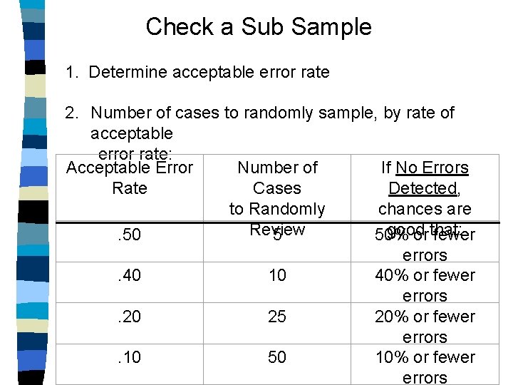
Check a Sub Sample 1. Determine acceptable error rate 2. Number of cases to randomly sample, by rate of acceptable error rate: Acceptable Error Number of If No Errors Rate Cases Detected, to Randomly chances are Review good. 50 5 50% or that: fewer errors. 40 10 40% or fewer errors. 20 25 20% or fewer errors. 10 50 10% or fewer errors

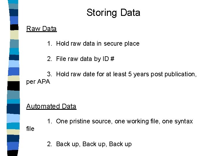
Storing Data Raw Data 1. Hold raw data in secure place 2. File raw data by ID # 3. Hold raw date for at least 5 years post publication, per APA Automated Data 1. One pristine source, one working file, one syntax file 2. Back up, Back up

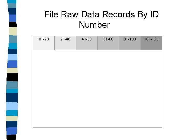
File Raw Data Records By ID Number 01 -20 21 -40 41 -60 61 -80 81 -100 101 -120

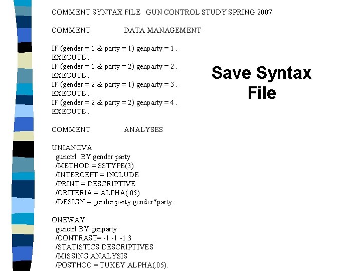
COMMENT SYNTAX FILE GUN CONTROL STUDY SPRING 2007 COMMENT DATA MANAGEMENT IF (gender = 1 & party = 1) genparty = 1. EXECUTE. IF (gender = 1 & party = 2) genparty = 2. EXECUTE. IF (gender = 2 & party = 1) genparty = 3. EXECUTE. IF (gender = 2 & party = 2) genparty = 4. EXECUTE. COMMENT ANALYSES UNIANOVA gunctrl BY gender party /METHOD = SSTYPE(3) /INTERCEPT = INCLUDE /PRINT = DESCRIPTIVE /CRITERIA = ALPHA(. 05) /DESIGN = gender party gender*party. ONEWAY gunctrl BY genparty /CONTRAST= -1 -1 -1 3 /STATISTICS DESCRIPTIVES /MISSING ANALYSIS /POSTHOC = TUKEY ALPHA(. 05). Save Syntax File