CARA Fault Tree Jrn Vatn http folk ntnu

CARA Fault. Tree Jørn Vatn http: //folk. ntnu. no/jvatn/ppt/CARAFault. Tree. ppt x

Content • Dag 1 – Gjennomgang feiltreanalyse som metode (definisjon av topphendelse, konstruksjon, minimale kuttmengder, kvalitativ og kvantitativ analyse) – Konstruksjon av feiltre i CARA Fault. Tree – Innlegging av pålitelighetsdata – Import/Eksport av pålitelighetsdata – Minimale kuttmengder – Frekvens og sannsynlighet for TOPP hendelsen – Mål for pålitelighetsmessig betydning • Dag 2 – – – Valg av analysetilnærminger (simulering, numerisk integrasjon mm) Innstillinger/valg Begrensninger i feiltreanalysen Kobling av feiltreanalyse og enkel MARKOV analyse Kobling feiltre og hendelsestreanalyse Bruk av Excel sammen med CARA Fault. Tree

What is a fault tree? • A fault tree is a logic diagram that displays the relationships between a potential critical event (accident) in a system and the reasons for this event • The reasons may be environmental conditions, human errors, normal events (events which are expected to occur during the life span of the system) and specific component failures • A properly constructed fault tree provides a good illustration of the various combinations of failures and other events which can lead to a specified critical event • The fault tree is easy to explain to engi neers without prior experience of fault tree analysis

What is a fault tree analysis (FTA)? • A fault tree analysis may be qualitative, quantitative or both, depending on the objectives of the analysis. Possible results from the analysis may e. g. be: – A listing of the possible combinations of environmental factors, human errors, normal events and component failures that can result in a critical event in the system. – The probability that the critical event will occur during a specified time interval – The most critical components in the system

FTA Procedure 1. Definition of the problem and the boundary condi tions. 2. Construction of the fault tree. 3. Identification of minimal cut sets. 4. Qualitative analysis of the fault tree. 5. Quantitative analysis of the fault tree.

1 Definition of the Problem and the Boundary Condi tions • Definition of the critical event (the accident) to be analysed. The critical event (accident) to be analysed is normally called the TOP event. • Definition of the boundary conditions for the analysis, i. e. , what to include (external power, sabotage etc) • To help defining the TOP event: – What: Describes what type of critical event (accident) is occur ring, e. g. collision between two trains. – Where: Describes where the critical event occurs, e. g. on a single track section. – When: Describes when the critical event occurs, e. g. during normal operation.

Example system

System description • In order to control the frequency of the turbine runner (TR) both servo motors (SM) have to function to put the guide vanes (GV) in correct position • The main distributing valve (MDV) is controlled by two servo valves (SV) • Each servo valve is a gain controlled by a programmable logical controller (PLC) via an input card (IPC) • It is sufficient that one servo valve with IPC and PLC is functioning in order to have the main distributing valve to operate • The oil pressure system (OPS) comprises both an oil tank, and an oil pump

Definition of the TOP event • What: Guide vanes (ledeskovler) in wrong position • Where: At the turbine runner • When: Under normal operation, i. e. , no system out for maintenance

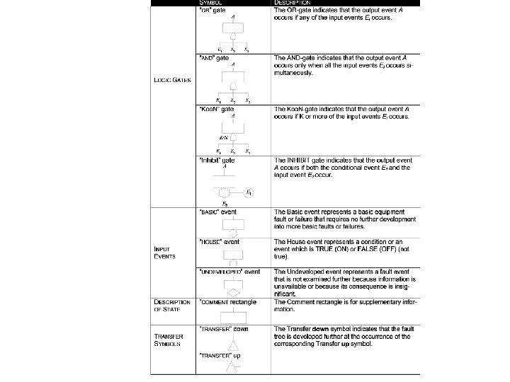
2. Construction of the Fault Tree 1. Start with the TOP event 2. Identify all fault events which are the im medi ate, necessary and sufficient causes that result in the TOP event (“What are the (direct) reasons for. . . ? ”) 3. Connect to the TOP event via a logic gate (AND or OR gate) 4. Proceed in the same manner with the gates until the “basic event” level is reached

Construction, Step 1 • TOP = Guide vanes in wrong position • Direct causes – Guide vanes stuck – Insufficient power from servo motors • Combine with OR gate

In CARA Fault. Tree

Exercise • Complete the analysis for the example case – Only qualitative input – No data – No analysis • Always ask for “what are the reasons for. . ? ”

CARA Fault. Tree pages • Use several pages if – The fault tree becomes large – The same system is included several places in the fault tree (physically the same) • Procedure – Add a Transfer Down – Right click | New Page – Change name of the new page

Naming conventions • Two symbols with the same name represent the same component • If two components are identical (same failure rate etc), but are two physical components, they should have different name, e. g. , PLC 1 and PLC 2 • When changing the name of a component, and giving the name of an existing component, you are prompted to verify this. The current component then gets data from the existing component

3 Identification of minimal cut sets • A fault tree provides valuable information about possible com binations of fault events which can result in a critical failure (TOP event) of the system • A cut set in a fault tree is a set of Basic events whose (simu ltaneous) occurrence ensures that the TOP event occurs • A cut set is said to be minimal if the set cannot be reduced without loosing its status as a cut set

4 Qualitative Evaluation of the Fault Tree • A qualitative evaluation of the fault tree may be carried out on the basis of the minimal cut sets • The importance of a cut set depends obviously on the number of Basic events in the cut set. The number of different Basic events in a minimal cut set is called the order of the cut set • A cut set of order one is usually more critical than a cut set of order two, or higher

4 Qualitative Evaluation of the Fault Tree, cont. • Another important factor is the type of Basic events in a minimal cut set • We may rank the criticality of the various cut sets according to the following ranking of the Basic events: 1. Human error 2. Failure of active equipment 3. Failure of passive equipment

5 Quantitative Analysis of the Fault Tree • When reliability data for each of the basic events is available, it is possible to carry out a quantitative evaluation of the fault tree. Different system reliability measures may be of interest: – Q 0(t) The proba bility that the TOP event occurs at time t – R 0(t) The probability that the TOP event does not occur in [0, t) – MTTF 0 Mean time to first system failure – F 0 TOP event frequency – I(i, t) Importance of component i at time t

Input data to the FTA • Quantitative result from a fault tree cannot be obtained unless failure data for each basic event is defined • Various types of data are used depending on the situation: – Frequency – On demand probability – Test interval – Repairable unit – Non repairable unit

Input data Category of failure data Reliability Parameters Frequency f = Frequency 1) On demand probabili ty q = Probability Test interval t* =Test interval 2), = Mean time to repair (MTTR) 2) and = Failure rate 3) Repairable unit = Mean time to repair 2) and = Failure rate 3) Non repair able unit = Failure rate 3) 1) 2) 3) Expected number of occurrences per 106 hours. Given in hours. Expected number of failures per 106 hours.

CARA Fault. Tree

Frequency • This category is used to describe events occurring now and then, but with no duration. Thus the probability that the event is occurring at time t, qi(t) = 0. • Note! If there is a duration of the event, the event should be described as a repairable unit, where the failure rate equals the frequency of the event, and the mean down time equals the duration

On demand probability • This category is usually used to describe components which is not activated during normal operation • The component is demanded only now and then • The reliability data represents the probability that the component is not able to perform its function upon request • In safety systems, the operator is often modelled by an on demand probability, for example: Operator fails to activate manual shut down system

Test interval •

Repairable and non repairable units • Repairable unit: The component is repaired when a failure occurs • Non repairable unit: It is not possible to repair the unit when a failure occurs (at least not within the analysis period)

Sharing data • In some situations many components are considered identical, i. e. , they have the same failure rate, MTTR etc • We may then define event classes to specify “look up” data:

Export data • Select File | Export data … to export data to a text file • The file can be imported into MS Excel:

CARA Fault. Tree reliability database • Since CARA Fault. Tree can import and export reliability data, it is possible to establish a reliability database which can easily be imported into a fault tree • Generic reliability data should be stored as “<event class>” • When the fault tree is completed qualitatively, one may import all reliability data from the database, given efficient naming convention

Q 0(t) The proba bility that the TOP event occurs at time t •

Q 0(t), cont •

Q 0(t) – “Upper bound” •

F 0 – TOP event frequency • We will demonstrate the method for calculating the TOP event frequency, F 0 in the following situation for each minimal cut set: – One and only one basic event is of the type ”frequency” with occurrence rate f – The remaining basic events is of the type “barrier/on demand probability”, with a barrier probability q

F 0 – Formulas •

Measures of Importance • The reliability importance of a component in a system will generally depend on the location of the component in the system, and the reliability of the component • A number of different measures are available in CARA Fault. Tree: – – – Vesely Fussell’s measure of reliability import ance. Birnbaum’s measure of reliability import ance. Improvement potential. Criticality Importance. Order of smallest cut set Birnbaum’s measure of structural import ance

Vesely Fussell • Vesely Fussell’s measure of reliability importance for component i is defined by: – IVF(i|t) = the conditional probability that at least one minimal cut set containing input event no. i is failed at time t, given that the system fails at time t • IVF(i|t) is rather simple to calculate

Birnbaum’s Measure • Birnbaum’s measure of reliability importance for component i is defined as follows – IB(i|t) = the partial derivative of Q 0(t) with respect to qi(t) • It can be shown that: – IB(i|t) = Pr(“TOP event occurs at t” | qi(t)=1) Pr(“TOP event occurs at t” | qi(t)=0) • It can also be shown that – IB(i|t) = The probability that component i is critical

Improvement potential • The improvement potential reliability measure for component i is defined by: – IIP(i|t) = the increase in system reliability if component i is replaced with a perfect component at time t

Criticality Importance • The criticality importance reliability measure for component i is defined by: – ICR(i|t) = the probability that component i is critical for the system and is failed at time t, given that the system is failed at time t.

Order of smallest cut set • The order of smallest cut set importance measure is defined by – IO(i) = The order of the smallest cut set containing component i

Systems with buffers • CARA Fault. Tree is not designed to treat buffer system • Some tricks exist • Consider the oil pressure system

Buffers, cont. • Assume the oil pressure tank has 8 hours capacity when fully charged • Upon a failure of the pump, the system will continue to support oil pressure for 8 hours • If a repair is conducted before 8 hours, no system disturbance will occur • What is the rate of failure of the oil pressure system, and what is the MTTR?

Buffers, cont • • Assume that MTTR for the pump is 4 hours Assume that = 400 (per million hours) Let p = Pr(TTR > buffer capacity) = e 8/4 The oil pressure system may now be modelled by: – System = Pump p – MTTRSystem = MTTRPump (TTR = Time To Repair)

UPS Buffer •

Fault tree

TOP event figures • Frequency of Top event (TOP): 9. 10398 e 006 [Occ. per Hours] • Unavailability [Qo(t)]: 9. 0849 e 005

Markov Analysis

Introduction • Markov analysis is used to model systems which have many different states • These states range from “perfect function” to a total fault state • The migration between the different states may often be described by a so called Markov model • The possible transitions between the states may further be described by a Markov diagram

Purpose • Markov analysis is well suited for deciding reliability characteristics of a system • Especially the method is well suited for small systems with complicated maintenance strategies • In a Markov analysis the following topics will be of interest – Estimating the average time the system is in each state. These numbers might further form a basis for economic considerations. – Estimating how frequent the system in average “visits” the various states. This information might further be used to estimate the need for spare parts, and maintenance personnel. – Estimate the mean time until the system enters one specific state, for example a critical state.

Markov Analysis procedure 1. Make a sketch of the system 2. Define the system states 3. Draw the Markov diagram with the transition rates 4. Quantitative assessment 5. Compilation and presentation of the result from the analysis

Make a sketch of the system • Pump system wit active pump and a spare pump in standby

Definition of system states • x 1 = state of active pump • x 2 = state of standby pump System state x. S Component state Comments x 1 x 2 2 1 1 Both pumps functioning 1 0 1 The active pump is in a fault state, the standby pump is functioning 0 0 0 Both pumps in a fault state

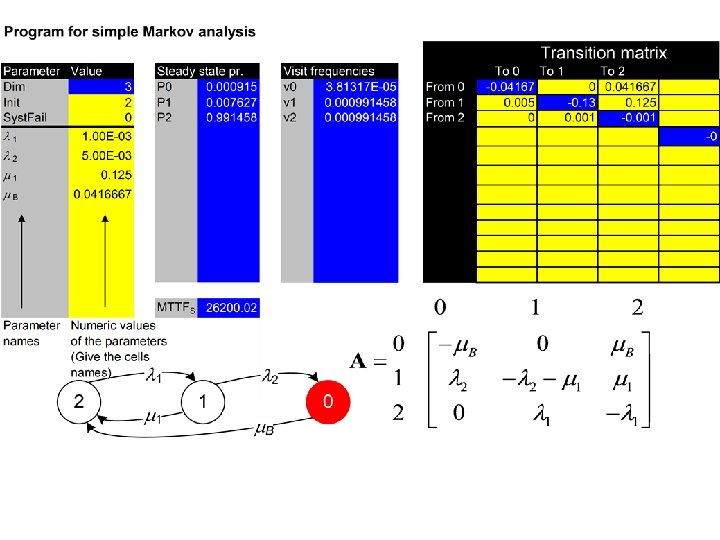
State transitions • • • 1 = 2 = 1 = B = For this system we have assumed that if the active pump fails, the standby pump could always be started Further we assume that if both pumps have failed, they will both be repaired before the system is put into service again The following transition rates are defined failure rate of the active pump failure rate of the standby pump (while running, 2 = 0 in standby position) repair rate of the active pump (1/ 1 = Mean Down Time when the active pump has failed) repair rate when both pumps are in a fault state. I. e. we assume that if the active pump has failed, and a repair with repair rate 1 is started, one will ”start over again” with repair rate B, if the standby pump also fails, independent of “how much” have been repaired on the active pump.

Markov state space diagram • The circles represent the system states, and the arrows represent the transition rates between the different system states • The Markov diagram and the description of states represent the total qualitative description of the system

Quantitative assessment • We want to assess the following quantities – Average time the system remain in the various system states – The visiting frequencies to each system state

Transition matrix • The indexing starts on 0, and moves to r, e. g. there are r +1 system states • Each cell in the matrix has two indexes, where the first (row index) represent the ”from” state, whereas the second (column index) represent the “to” state. • The cells represent transition rates from one state to another • aij is thus the transition rate from state i to state j • The diagonal elements are a kind of ”dummy” elements, which are filled in at the end, and shall fulfil the condition that all cells in a row adds up to zero

Example transition matrix: (From , To )

State probabilities • Let Pi(t) represent the probability that the system is in state i at time t • Now introduce vector notation, i. e. • P(t) = [P 0(t), P 1(t), …, Pr(t)] • From the definition of the matrix diagram it might be shown that the Markov state equations are given by: P(t) A = d P(t)/d t • These equations may be used to establish both the steady state probabilities, and the time dependent solution

Steady state probabilities • Let the vector P = [P 0, P 1, …, Pr] represent the average time the system is in the various system states in the long time run • For example, P 0 is average fraction of the time the system is in state 0, P 1 is average fraction of the time the system is in state 1 • The elements P = [P 0, P 1, …, Pr] are also denoted steady state probabilities to indicate that in the stationary situation Pi represents the probability that the system is in state i.

The steady state solution • In the long run when the system has stabilized we must have that d P(t)/d t = 0, hence • P A = 0 • This system of equations is over determined, hence we may delete one column, and replace it with the fact that P 0+ P 1+…+Pr = 1 • Hence, we have

The steady state solution P A 1 = b where and b = [0, 0, …, 0, 1]

Example which gives

Numerical solution • To solve the steady state equations P A 1 = b is a tedious task • Often we therefore solve these equations by numerical methods • The Markov. xls program does this, where we have to: – Define the transition rates – Assign numerical values to the transition rates – Specify the Markov state space matrix

Visiting frequencies • Often we are interested in evaluating how many times the system enters the various states, i. e. the visiting frequencies • The visiting frequency for state j is denoted j, and could be obtained by: • j = Pj ajj • From our example we obtain the “system failure rate”

Time dependent solution • Up to now we have investigated the steady state situation • In some situations we also want to investigate the time dependent solution, i. e. the probability that the system is in e. g. state 0 at time t • We now let Pi(t) be the probability that the system is in state i at time t • The time dependent solution may be found by: • P(t) A = d P(t)/d t • Which could be solved by Laplace methods, or numerical methods • For numerical methods we apply Markov. xls

Standby generator • Consider a system with fed by a public net • The failure rate and repair rate of the net is N and N • A generator is installed as a cold backup in case of failure of the public net • In passive mode the generator has a failure rate G, 0, and in active mode the failure rate is G, and the repair rate is G • In standby mode the generator is tested with intervals of length to reveal hidden fail to start failures

Simplified Markov diagram • From Markov analysis – – – 0 = Visiting frequency to state 0 0 to be used as failure rate ( ) in FTA P 0 = Steady state probability of state 0 MDT 0 = Mean sojourn time in state 0 MDT 0 P 0 / 0 to be used as MTTR in FTA • http: //folk. ntnu. no/jvatn/Computer. Programs/Markov. Standby. Generator. xls

Exact Markov diagram • State 3 = Net restored before standby generator is repaired

The “net” is more than one component: • Assume that the external net is modelled by e. g. , a fault tree • This means that we need to find N and N from the FTA • We then use – N = F 0 /Q 0, since Q 0 N / N • N and N is then input to the Markov, which again is input to the detailed FTA on the cite