An Introduction to Rheology and Its Applications Complex

流變學之簡介與應用 An Introduction to Rheology and Its Applications Complex Fluids & Molecular Rheology Lab. , Department of Chemical Engineering

課程大綱 I. 流變現象與無因次群分析 II. 基礎量測系統與功能 III. 影響流變行為的主要因素 IV. 實驗分析原理與技術 Principal References: “Dynamics of Polymeric Liquids: Volume 1 Fluid Mechanics” by R. B. Bird et al. , 2 nd Ed. , Wiley-Interscience (1987)

什 麼 是 流 變 (Rheology)? o Rheology is the science of fluids. More specifically, the study of Non-Newtonian Fluids Newton’s law of viscosity 牛頓流體 - 水、有機小分子溶劑等 黏度η為定值 o 流體 非牛頓流體 - 高分子溶液、膠體等 黏度不為定值 (尤其在快速流場下) o 為何需要流變學家? § § Macromolecules are easily deformable Chain interactions are complicated Processings typically involve flows Try to make Rheology not an issue

非牛頓流體的特徵 o 非牛頓黏度 (Non-Newtonian Viscosity) - Shear Thinning Flow curve for non-Newtonian Fluids 牛頓流體 (甘油加水) 非牛頓流體 (高分子溶液)

o 記憶效應 (Memory effects) - Elastic Recoil - Open Syphon Flow

牛 頓 流 體 的 不 穩 定 性: 慣 性 效 應 Concentric Cylinders Onset of Secondary Flow Ta (or Re) plays the central role! Laminar Secondary Turbulent Taylor vortices Turbulent

流 變 性 質 的 微 觀 (分 子) 成 因 o 微觀的角度 ● ● Small molecule Deformable Macromolecule o 流變的性質主要決定於 流體組成性質 流場因素 Dilute/Entangled Polydispersity Flexibility Linear/Branched Chain interactions Flow strength Flow kinematics Competition between relaxation & deformation rates

o 典型製程之流場強度範圍 Lubrication High-speed coating Rolling Spraying Injection molding Pipe flow Chewing Extrusion Sedimentation Typical viscosity curve of a polyolefin- PP homopolymer, melt flow rate (230 C/2. 16 Kg) of 8 g/10 minat 230 C with indication of the shear rate regions of different conversion techniques. [Reproduced from M. Gahleitner, “Melt rheology of polyolefins”, Prog. Polym. Sci. , 26, 895 (2001). ]

Secondary Flows and Instabilities o Secondary flow around a rotating sphere in a polyacrylamide solution. [Reporduce from H. Giesekus in E. H. Lee, ed. , Proceedings of the Fourth International Congress on Rheology, Wiley-Interscience, New York (1965), Part 1, pp. 249 -266]

o Melt instability Sharkskin Melt fracture Photographs of LLDPE melt pass through a capillary tube under various shear rates. The shear rates are 37, 112, 750 and 2250 s-1, respectively. [Reproduced from R. H. Moynihan, “The Flow at Polymer and Metal Interfaces”, Ph. D. Thesis, Department of Chemical Engineering, Virginia Tech. , Blackburg, VA, 1990. ] [Retrieved from the video of Non-Newtonian Fluid Mechanics (University of Wales Institute of Non-Newtonian Fluid Mechanics, 2000)]

o Taylor-Couette flow for dilute solutions Taylor vortex R 1 R 2 [S. J. Muller, E. S. G. Shaqfeh and R. G. Larson, “Experimental studies of the onset of oscillatory instability in viscoelastic Taylor-Couette flow”, J. Non-Newtonian Fluid Mech. , 46, 315 (1993). ] Flow visualization of the elastic Taylor-Couette instability in Boger fluids. [http: //www. cchem. berkeley. edu/sjmgrp/]

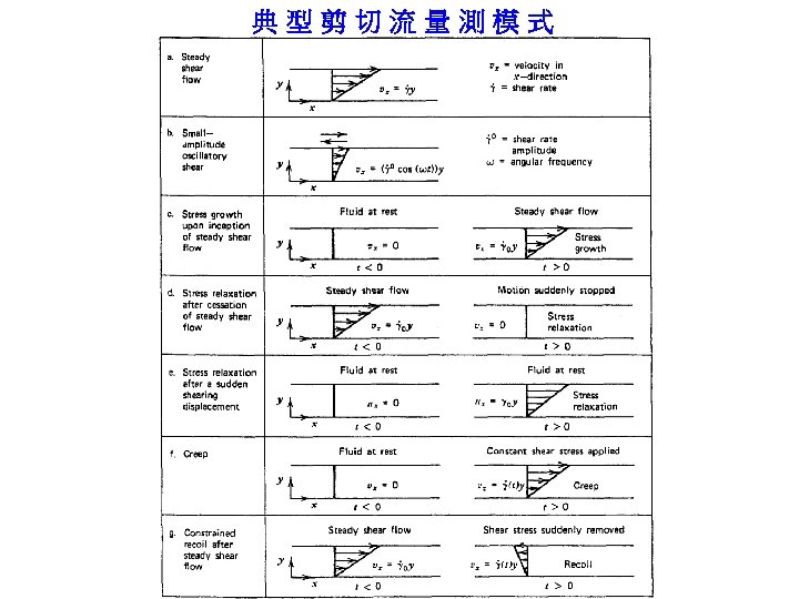
典型均勻流場 q Two standard types of flows, shear and shearfree, are frequently used to characterize polymeric liquids (a) Shear (b) Shearfree Steady simple shear flow Shear rate Streamlines for elongational flow (b=0) Elongation rate

q The Stress Tensor y x Shear Flow Total stress tensor* Stress tensor Hydrostatic pressure forces z Elongational Flow

q流 變 儀 夾 具 與 流 場 特 性 (a) Shear Pressure Flow: Capillary Drag Flows: Concentric Cylinder (b) Elongation Cone-and. Plate Moving Parallel Plates

q適 用 流 場 強 度 與 濃 度 範 圍 (a) Shear Concentrated Regime Homogeneous deformation: * Nonhomogeneous deformation: (b) Elongation Cone-and. Plate Parallel Plates Dilute Regime Concentric Cylinder Capillary Moving clamps For Melts & High-Viscosity Solutions *Stress and strain are independent of position throughout the sample

q基 礎 黏 度 量 測 Concentric Cylinder FIG. Concentric cylinder viscometer (homogeneous)

Cone-and-Plate Instrument (From p. 205 of ref 3) (homogeneous) FIG. 1. 3 -4. Cone-and-plate geometry

Uniaxial Elongational Flow Device used to generate uniaxial elongational flows by separating Clamped ends of the sample

I. 穩態剪切流 Exp a: Steady Shear Flow Non-Newtonian viscosity η of a low-density polyethylene at several Different temperatures The first and second normal stress The shear-rate dependent viscosity η coefficients are defined as follows: is defined as:

Relative Viscosity: Master curves for the viscosity and first normal stress difference coefficient as functions of shear rate for the low-density polyethylene melt shown in previous figure Intrinsic Viscosity: Intrinsic viscosity of dilute polystyrene Solutions, With various solvents, as a function of reduced shear rate β

II. 小振幅反覆式剪切流: 黏性與彈性檢定 Exp b: Small-Amplitude Oscillatory Shear Flow Oscillatory shear strain, shear rate, shear stress, and first normal stress difference in small-amplitude oscillatory shear flow

It is customary to rewrite the above equations to display the in-phase and out-of-phase parts of the shear stress Storage modulus Loss modulus Storage and loss moduli, G’ and G”, as functions of frequency ω at a reference temperature of T 0=423 K for the low-density polyethylene melt shown in Fig. 3. 3 -1. The solid curves are calculated from the generalized Maxwell model, Eqs. 5. 2 -13 through 15

III. 拉 伸 流 黏 度 量 測 與 特 徵 q Shearfree Flow Material Functions

The number average and weight average molecular weights of the samples: Monodisperse, but with a tail in high M. W. (GPC results)

I. 時間－溫度 疊合原理 (Time-Temperature Superposition) Non-Newtonian viscosity of a low-density polyethylene melt at several different temperatures. Master curves for the viscosity and first normal Stress coefficient as functions of shear rate for a low-density polyethylene melt

According to the Reptation Theory: Newtonian Zero-shear viscosity, 0 Power law

WLF 溫度重整因子: o Time-temperature superposition holds for many polymer melts and solutions, as long as there are no phase transitions or other temperature-dependent structural changes in the liquid. o Time-temperature shifting is extremely useful in practical applications, allowing one to make prediction of time-dependent material response.

WLF temperature shift parameters J. D. Ferry, Viscoelastic Properties of Polymers, 3 rd ed. , Wiley: New York (1980).

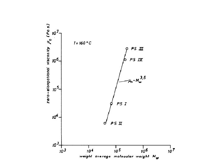
II. 分子量的效應 (Molecular Weight Dependences) For linear polymer melts Molecular weight, Mw Zero-shear Relaxation Diffusivity, viscosity, time, DG 0 < Mc ~ Mw ~ M w 2 ~ 1/Mw > Mc ~ Mw 3. 4 ~ M w 3 ~ 1/Mw 2 Mc (=2 Me): critical molecular weight Me: entangled molecular weight Plot of constant + log 0 vs. constant + log M for nine different polymers. The two constants are different for each of the polymers, and the one appearing in the abscissa is proportional to concentration, which is constant for a given undiluted polymer. For each polymer the slopes of the left and right straight line regions are 1. 0 and 3. 4, respectively. [G. C. Berry and T. G. Fox, Adv. Polym. Sci. 5, 261 -357 (1968). ]

A “Time-Temperature-Molecular Weight-Concentration” Superposition: A master curve of polystyrene-n-butyl benzene solutions. Molecular weights varied from 1. 6 x 105 to 2. 4 x 106 g/mol, concentration from 0. 255 to 0. 55 g/cm 3, and temperature from 303 to 333 K.

III. 分子量分佈的影響 H. Munstedt, J. Rheol. 24, 847 -867 (1980)

IV. 高分子結構的影響 (Molecular Architecture) Linear Polymer Star Polymer Pom-Pom Polymer polybutadiene Polyisoprene C. C. Hua, H. Y. Kuo, J Polym Sci Part B: Polym Phys 38, 248 -261 (2006) S. C. Shie, C. T. Wu, C. C. Hua, Macromolecules 36, 2141 -2148 (2003)

V. 溶劑品質及其對高分子溶液的影響 (Effects of Solvent Quality for Polymer Solutions) [cf. p 109] An example of viscosity versus concentration plots for polystyrene (Mw=7. 14 106 g/mol) in benzene at 30 C. White circles: plot of sp / c vs. c; black circles: plot of (ln r)/c vs. c. (1) Zimm-Crothers viscometer (3. 7 10 -3 ~7. 6 10 -2 dyn/cm 2); (2)Ubbelohde viscometer (8. 67 dyn/cm 2); (3)Ubbelohde viscometer (12. 2 dyn/cm 2). T. Kotaka et al. , J. Chem. Phys. 45, 2770 -2773 (1966).

Superposition of Intrinsic Viscosity Data on Various Solvent Systems: ØMagnitude of intrinsic viscosity Ø -temperature & Solvent ØFlow curve T. Kotaka et al. , J. Chem. Phys. 45, 2770 -2773 (1966).

Essential Scaling Laws: o The solvent quality is an index describing the strength of polymer-solvent interactions. o This interaction strength is a function of chemical species of polymer & solvent molecules, temperature, and pressure. Scaling law of polymer size and molecular weight (<R 2>end-to-end 1/2 ~ Mw ). Root mean square end-to-end distance Solvent condition Good <R 2>end-to-end 1/2 Bad Temperature T T> T= T< Index 3/5 1/2 1/3

Phase Separation by Temperature-Induced Solvent Quality Changes: The (temperature, weight fraction) phase diagram for the polystyrene-cyclohexane system for samples of Indicated molecular weight. S. Saeki et al, Macromolecules 6, 246 -250(1973). TU: upper critical solution temperature TL: lower critical solution temperature

Coil-Globule Transition due to Changes in Solvent Quality: Poly(N-isopropylacrylamide) in water Mw = 4. 45 x 105 g/mol, c = 6. 65 x 10 -4 g/ml Mw = 1. 00 x 107 g/mol, c = 2. 50 x 10 -5 g/ml coil globule X. Wang et al. , Macromolecules 31, 2972 -2976 (1998). H. Yang et al. , Polymer 44, 7175 -7180 (2003).

I. 線性黏彈性分析 (Linear Viscoelasticity) o The Maxwell model (for melts or concentrated solutions) The nature of flow Relaxation modulus, G(t): The nature of fluid

Other Transformation Relationships s = t-t’ η 0 is zero-shear viscosity η’ is dynamic viscosity Je 0 is steady- state compliance

G 0 G(t) (Pa) The single exponential mode, eq 1, with relaxation time λ=0. 1 s and G 0=105 Pa. The single mode dose not fit typical data well. A logical improvement on this model is to try several relaxation times , shown as eq 2. G 1 G(t) (Pa) G 2 G 3 G 4 G 5 C. H. Macosko, Rheology Principles, Measurements, and Applications, Wiley-VCH: New York (1994). t (s) A spectral decomposition of five-constant model combined with eq 2.

G”(Pa) Relaxation times and moduli for LDPE at 150℃ λk (s) Gk (Pa) 1 103 1. 00 2 102 1. 80× 102 3 10 1. 89× 103 4 100 9. 80× 103 5 10 -1 2. 67× 104 6 10 -2 5. 86× 104 7 10 -3 9. 48× 104 8 10 -4 1. 29× 105 G’(Pa) k ω(s-1) Dynamic shear moduli for LDPE at 423 K. Data were collected at different temperatures and shifted according to time-temperature superposition. The solid curves are calculated from G(t) using eq 1 -2. Spectral decomposition of the storage and loss moduli for LDPE at 423 K. The moduli are calculated by eq 1 -2 with the Gk and λk given in left table.

線性黏彈性實驗數據轉換法則 (Transformation between linear viscoelastic data) The Cox-Merz rule Flow geometry : Cone and plate (25 mm diameter, cone angle 2 °) Material properties for PS solutions Sample Mw (10 -6 g PDI Solvent /mol) Wt % Zeq η 0 (Pa．s) Je 0 (Pa-1) τrep (s) T (k) PS 2 Ma 7 6. 5 1. 73× 104 6. 33 298 3. 66× 10 -4 η + (Pa s) DEP η, η* (Pa s) G’, G” (pa) 1. 09 ． 2. 0 ． t (s) ω (1/s) Dynamic moduli measured in small-amplitude oscillatory experiments for a monodisperse solution PS 2 Ma: measurements were conducted at 25℃ Comparison between steady-shear and complex viscosities for a monodisperse solution, PS 2 Ma: measurements were conducted at 25℃ Transient viscosity growth for a monodisperse solution, PS 2 Ma, following startup of steady shearing at various shear rates; measurements were conducted at 25 ℃ Y-H Wen, H-C Lin, C-H Li, C-C. Hua, Poymer 45, 8551 -8559

Laun’s rule a was original given as 0. 7 Material properties for PS solutions Flow geometry : Cone and plate (25 mm diameter, cone angle 2 °) PDI Solvent Wt % Zeq η 0 (Pa．s) Je 0 (Pa-1) τrep (s) T (k) PS 2 Mb 2. 0 1. 09 DEP 20 32. 2 1. 17× 105 6. 0× 10 -4 70. 2 313 Transient behavior of first normal stress difference coefficient for a monodisperse solution, PS 2 Mb, following startup of steady shearing at various shear rates; measurements were conducted at 40 ℃ Ψ 1 (Pa. s 2) Mw (10 -6 g /mol) Ψ 1 (Pa. s 2) Sample Comparison between experimentally measured first normal stress difference coefficient(points) and predictions (lines) based on Laun’s rule for a monodisperse solutions, PS 2 Mb; measurements were conducted at 40 ℃ Y-H Wen, H-C Lin, C-H Li, C-C. Hua, Poymer 45, 8551 -8559

基礎流變參數的取得 (Retrieval of Fundamental Material Constants from Linear Viscoelastic Data) e ~ M 0 d ~ M 3 Storage modulus vs. frequency for narrow distribution polystyrene melts. Molecular weight ranges from Mw = 8. 9 x 103 r/mol (L 9) to Mw = 5. 8 x 105 g/mol (L 18). Theoretical results of (a) G(t) and (b) G’( ) for polymer melts. M. Doi and S. F. Edwards, Theory of Polymer Dynamics, Oxford Science: New York (1986), pp 229 -230.

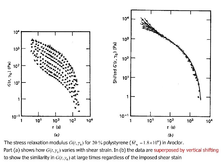
Stress Relaxation after a Sudden Shearing Displacement (Step-Strain Stress Relaxation) Relaxation Modulus: * For small shear strains The Lodge-Meissner Rule:

II. 非線性黏彈性分析 (Nonlinear Viscoelasticity) Determination of model parameters Flow geometry : Cone and plate (25 mm diameter and cone angle 4 °) Essential model parameters and time constants Sample PS/DEP Zeq τe (s) τR (s) τd, 0 (s) τi (s) 42 2. 0 × 10 -4 0. 71 89. 4 0. 157 G’ and G” (Pa) Set 3 Solution (Pa) 5. 0 × 103 Zeq : number of entanglements Φ : polymer volume fraction Me, melt = 13, 300 for PS, α = 1. 3 Experiment (Set 3) τ e = 2. 0 × 10 -4 s; Zeq = 42 ω (1/s) Y. H. Wen, C. C. Hua, J Polym Sci Part B: Polym Phys 44, 1199 -1211 (2006)

Tube model formulation for single – step strain flows Properties of relaxation modes utilized to fit linear stress relaxation data Set 3 F(t) : the time-dependent tube survival probability describing the linear stress relaxation. Plateau modulus λ (t) : Primitive chain length normalized by its equilibrium value Qyx(γ) : the yx component of the orientation tensor Stretch relaxation of a 1 -D Rouse chain gi λi 0. 1989 0. 133 0. 1579 0. 275 0. 0859 0. 571 0. 1820 1. 19 0. 0816 2. 46 0. 1377 5. 11 0. 0841 10. 6 0. 0643 22. 0 0. 0029 45. 8 0. 0055 95. 0 The first term in eq. A 14 may be plausibly described as arising from the contribution of local segmental-length fluctuation. The second term in eq. A 14 represents the contribution from the fluctuations of entire chain length.

G(t, γ) (Pa) Theory /data comparison for nonlinear stress relaxation t (s)

Linear viscoelastic measurements for elongational flow properties G’ Slope: ne G” Baumgaertel, Schausberger, and Winter (BSW) model Slope: ng PS 390 K: closed symbols PS melt properties at 130 ℃ Mw (g/mol) Mw/Mn λ 0 (s) 3. 9× 105 1. 06 h(x) is the Heaviside step function H 1 describes the rubbery behavior at low and intermediate ω, while H 2 describes the glassy behavior at large ω 2. 1× 104 ne 0. 16 ng 0. 7 H 1λ 0 ne (Pa) 4. 17× 104 H 2λ 0 -ng (Pa) 20 (k. Pa) 257 η 0 (MPa s) 755 A. Bach, K. Almdal, H. K. Rasmussen, O. Hassager, Macromolecules 36, 5174 -5179 (2003)

3 η 0 PS 390 K A. Bach, K. Almdal, H. K. Rasmussen, O. Hassager, Macromolecules 36, 5174 -5179 (2003)