ADVANCED COMPUTER ARCHITECTURE ML Accelerators Samira Khan University

ADVANCED COMPUTER ARCHITECTURE ML Accelerators Samira Khan University of Virginia Feb 6, 2019 The content and concept of this course are adapted from CMU ECE 740

AGENDA • Review from last lecture • ML accelerators 2

LOGISTICS • Project list – Posted in Piazza – Please talk to me if you do not know what to pick – Please talk to me you have some idea for the project • Sample project proposals from many different years – Posted in Piazza • Project Proposal Due on Feb 11, 2019 • Project Proposal Presentations: Feb 13, 2019 – Can can present using your own laptop • Groups: 1 or 2 students 3

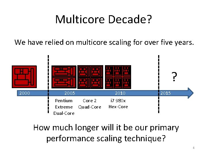
Multicore Decade? We have relied on multicore scaling for over five years. ? 2000 2005 Pentium Core 2 Extreme Quad-Core Dual-Core 2010 i 7 980 x Hex-Core 2015 How much longer will it be our primary performance scaling technique? 4

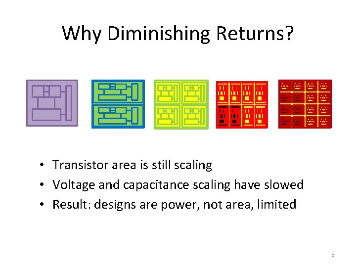
Why Diminishing Returns? • Transistor area is still scaling • Voltage and capacitance scaling have slowed • Result: designs are power, not area, limited 5

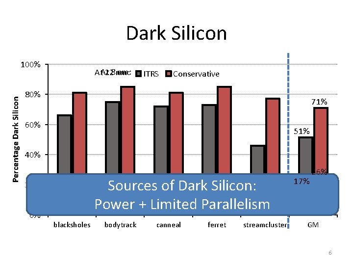
Dark Silicon Percentage Dark Silicon 100% nm: At. At 228 nm: ITRS Conservative 80% 71% 60% 51% 40% Sources of Dark Silicon: Power + Limited Parallelism 20% 0% blacksholes bodytrack canneal ferret streamcluster 17% 26% GM GM 6

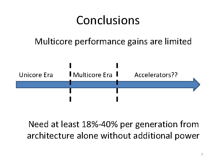
Conclusions Multicore performance gains are limited Unicore Era Multicore Era Accelerators? ? Need at least 18%-40% per generation from architecture alone without additional power 7

NN Accelerators 8

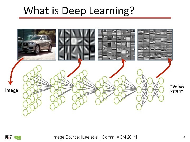
What is Deep Learning? “Volvo XC 90” Image Source: [Lee et al. , Comm. ACM 2011] 17

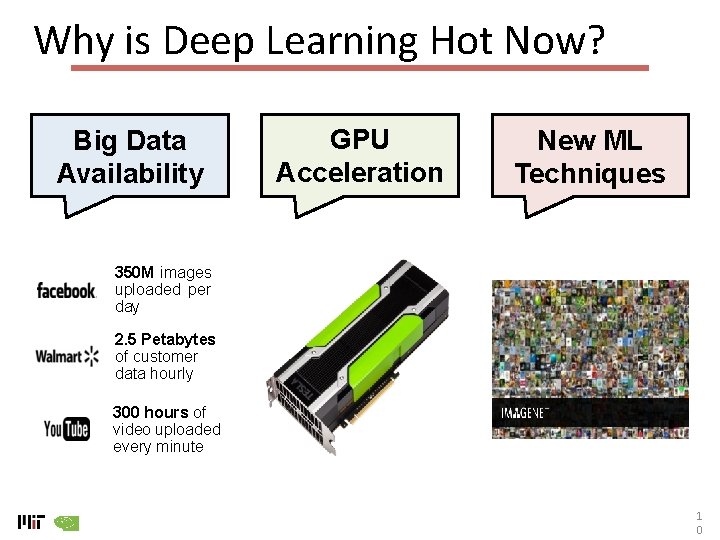
Why is Deep Learning Hot Now? Big Data Availability GPU Acceleration New ML Techniques 350 M images uploaded per day 2. 5 Petabytes of customer data hourly 300 hours of video uploaded every minute 1 0

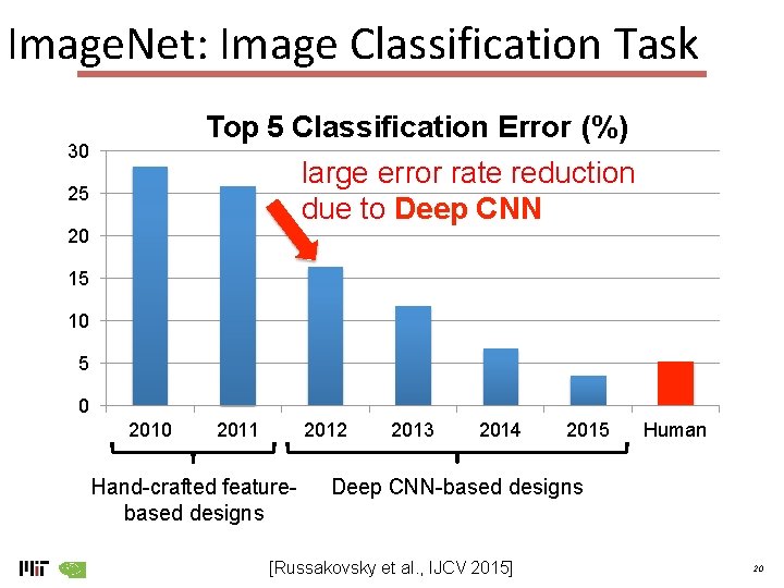
Image. Net: Image Classification Task Top 5 Classification Error (%) 30 large error rate reduction due to Deep CNN 25 20 15 10 5 0 2011 2012 Hand-crafted featurebased designs 2013 2014 2015 Human Deep CNN-based designs [Russakovsky et al. , IJCV 2015] 20

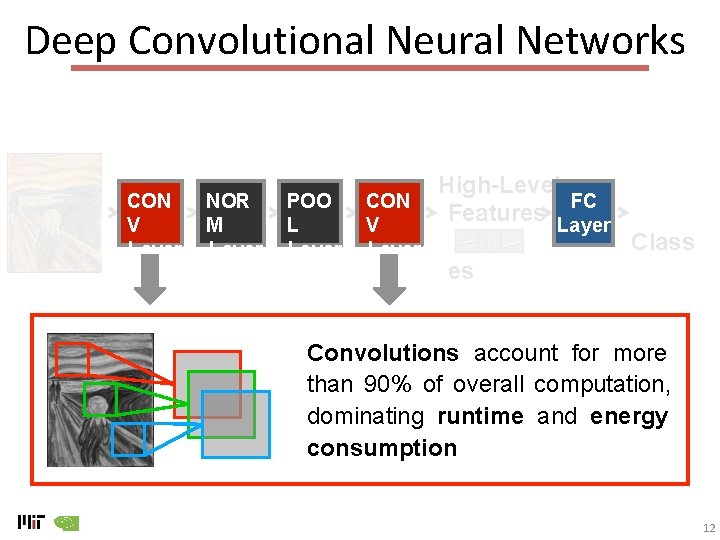
Deep Convolutional Neural Networks CON V Layer NOR M Layer POO L Layer CON V Layer High-Level FC Features Layer Class es Convolutions account for more than 90% of overall computation, dominating runtime and energy consumption 12

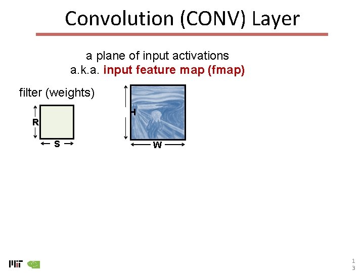
Convolution (CONV) Layer a plane of input activations a. k. a. input feature map (fmap) filter (weights) H R S W 1 3

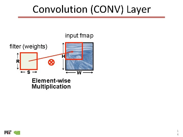
Convolution (CONV) Layer input fmap filter (weights) H R S W Element-wise Multiplication 1 4

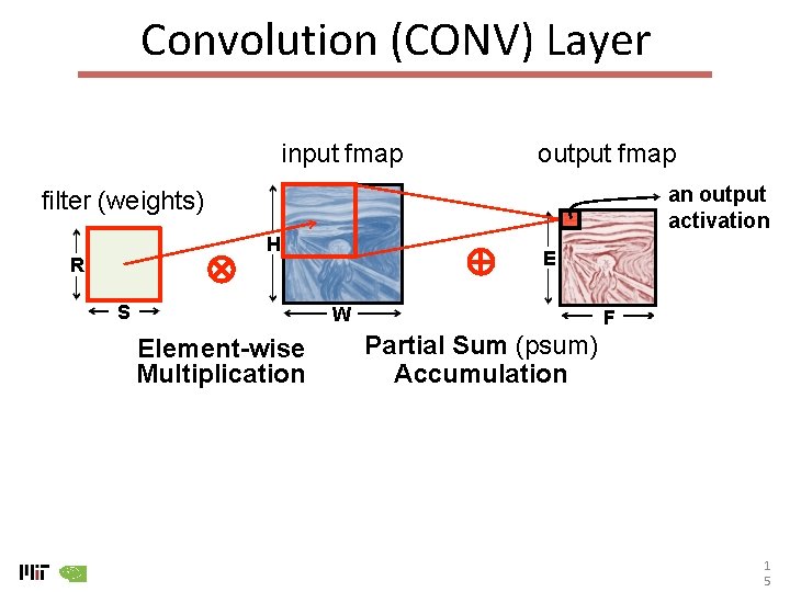
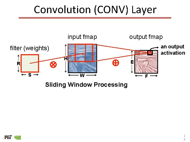
Convolution (CONV) Layer input fmap output fmap an output activation filter (weights) H R S E W Element-wise Multiplication F Partial Sum (psum) Accumulation 1 5

Convolution (CONV) Layer input fmap output fmap an output activation filter (weights) H R S E W F Sliding Window Processing 1 6

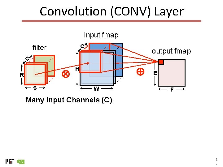
Convolution (CONV) Layer input fmap C filter output fmap C H R S E W F Many Input Channels (C) 1 7

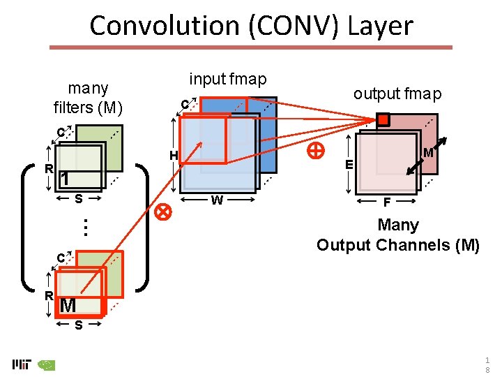
Convolution (CONV) Layer input fmap many filters (M) output fmap C C R H … C R E 1 S M W F Many Output Channels (M) M S 1 8

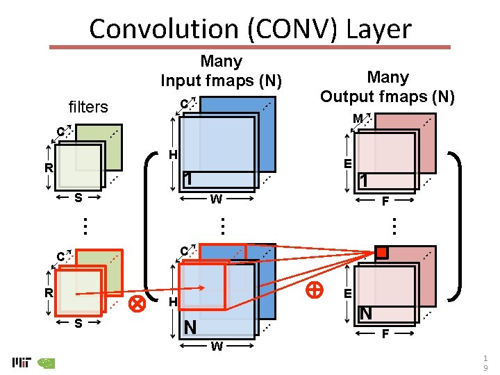
Convolution (CONV) Layer Many Input fmaps (N) C filters Many Output fmaps (N) M C H E 1 S 1 F … … W … R C C R E H S N N W F 1 9

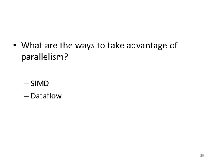
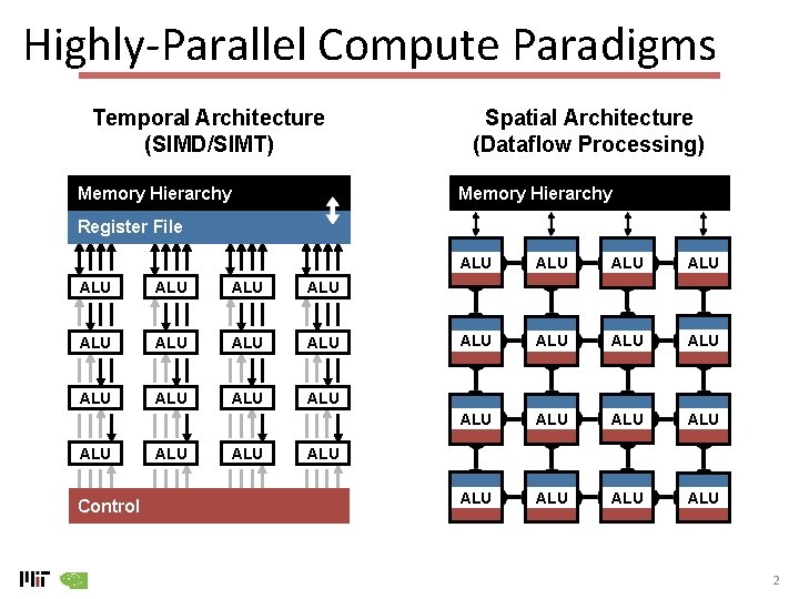
• What are the ways to take advantage of parallelism? – SIMD – Dataflow 20

Highly-Parallel Compute Paradigms Temporal Architecture (SIMD/SIMT) Memory Hierarchy Spatial Architecture (Dataflow Processing) Memory Hierarchy Register File ALU ALU ALU ALU Control ALU ALU ALU ALU ALU 2

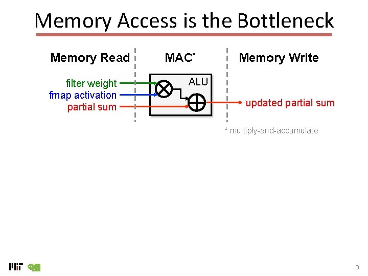
Memory Access is the Bottleneck Memory Read filter weight fmap activation partial sum MAC* Memory Write ALU updated partial sum * multiply-and-accumulate 3

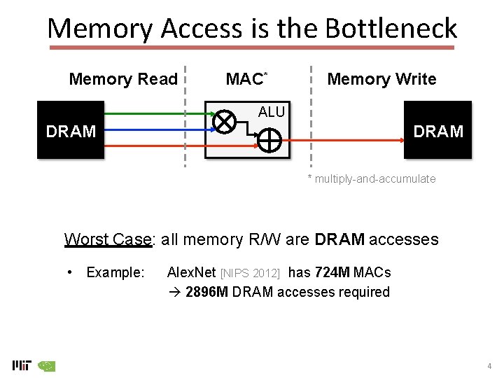
Memory Access is the Bottleneck Memory Read MAC* Memory Write ALU DRAM * multiply-and-accumulate Worst Case: all memory R/W are DRAM accesses • Example: Alex. Net [NIPS 2012] has 724 M MACs 2896 M DRAM accesses required 4

• What are the ways to address memory bottleneck? – Memory Hierarchy – Exploit locality 24

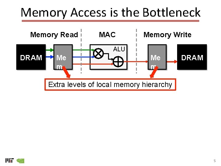
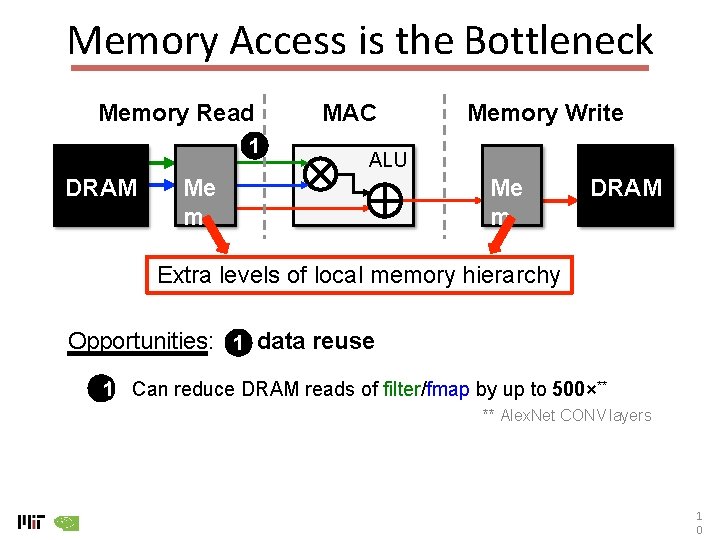
Memory Access is the Bottleneck Memory Read MAC Memory Write ALU DRAM Me m DRAM Extra levels of local memory hierarchy 5

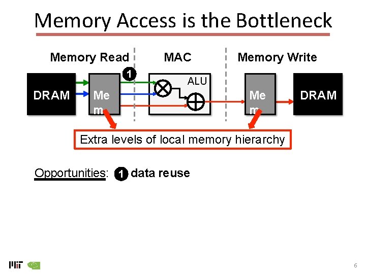
Memory Access is the Bottleneck Memory Read 1 DRAM MAC Memory Write ALU Me m DRAM Extra levels of local memory hierarchy Opportunities: 1 data reuse 6

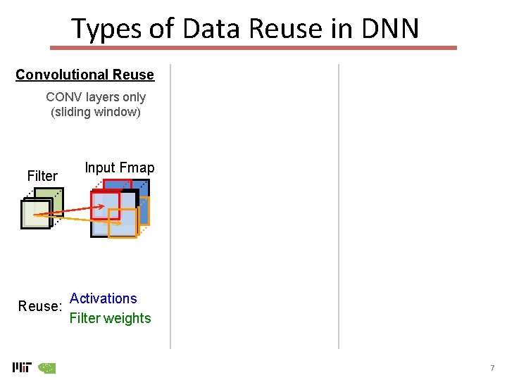
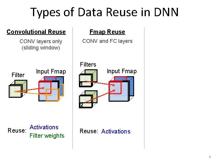
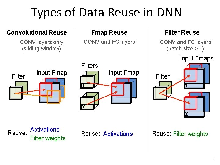
Types of Data Reuse in DNN Convolutional Reuse CONV layers only (sliding window) Filter Reuse: Input Fmap Activations Filter weights 7

Types of Data Reuse in DNN Convolutional Reuse CONV layers only (sliding window) Fmap Reuse CONV and FC layers Filter Input Fmap 1 2 Reuse: Activations Filter weights Reuse: Activations 8

Types of Data Reuse in DNN Convolutional Reuse CONV layers only (sliding window) Fmap Reuse CONV and FC layers Filter Reuse CONV and FC layers (batch size > 1) Input Fmaps Filter Input Fmap 1 Filter 1 2 2 Reuse: Activations Filter weights Reuse: Activations Reuse: Filter weights 9

Memory Access is the Bottleneck Memory Read 1 DRAM MAC Memory Write ALU Me m DRAM Extra levels of local memory hierarchy Opportunities: 1 data reuse 11) Can reduce DRAM reads of filter/fmap by up to 500×** ** Alex. Net CONV layers 1 0

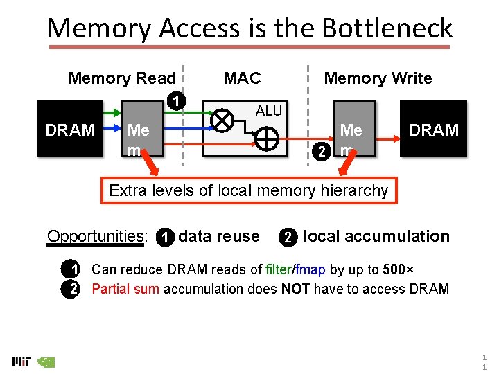
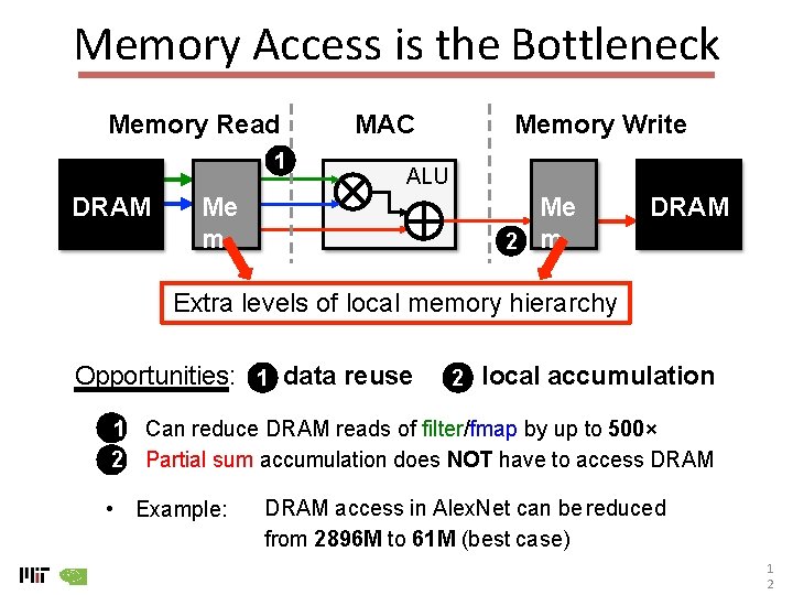
Memory Access is the Bottleneck Memory Read 1 DRAM MAC Memory Write ALU Me m Me 2 m DRAM Extra levels of local memory hierarchy Opportunities: 1 data reuse 2 local accumulation 11) Can reduce DRAM reads of filter/fmap by up to 500× 22) Partial sum accumulation does NOT have to access DRAM 1 1

Memory Access is the Bottleneck Memory Read 1 DRAM MAC Memory Write ALU Me m Me 2 m DRAM Extra levels of local memory hierarchy Opportunities: 1 data reuse 2 local accumulation 11) Can reduce DRAM reads of filter/fmap by up to 500× 22) Partial sum accumulation does NOT have to access DRAM • Example: DRAM access in Alex. Net can be reduced from 2896 M to 61 M (best case) 1 2

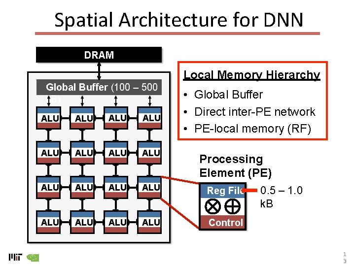
Spatial Architecture for DNN DRAM Local Memory Hierarchy Global Buffer (100 – 500 k. B) • Global Buffer • Direct inter-PE network • PE-local memory (RF) ALU ALU ALU Reg File ALU ALU Control Processing Element (PE) 0. 5 – 1. 0 k. B 1 3

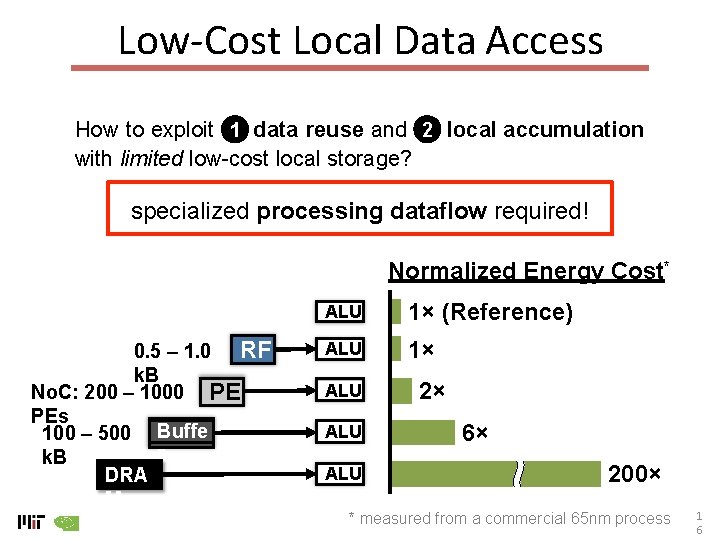
Low-Cost Local Data Access How to exploit 1 data reuse and 2 local accumulation with limited low-cost local storage? specialized processing dataflow required! Normalized Energy Cost* 0. 5 – 1. 0 RF k. B No. C: 200 – 1000 PE PEs 100 – 500 Buffe r k. B DRA M ALU 1× (Reference) ALU 1× ALU ALU 2× 6× 200× * measured from a commercial 65 nm process 1 6

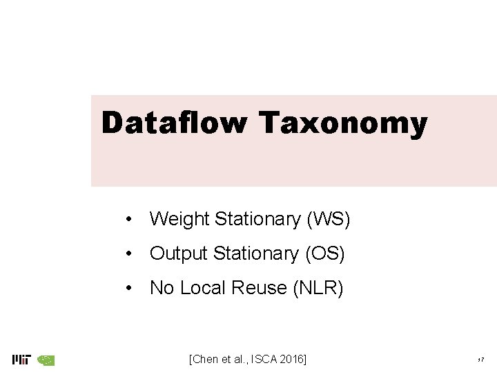
Dataflow Taxonomy • Weight Stationary (WS) • Output Stationary (OS) • No Local Reuse (NLR) [Chen et al. , ISCA 2016] 17

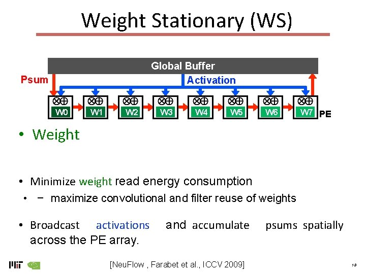
Weight Stationary (WS) Global Buffer Activation Psum W 0 W 1 W 2 W 3 W 4 W 5 W 6 W 7 PE • Weight • Minimize weight read energy consumption • − maximize convolutional and filter reuse of weights • Broadcast activations across the PE array. and accumulate [Neu. Flow , Farabet et al. , ICCV 2009] psums spatially 18

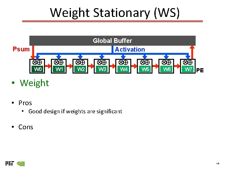
Weight Stationary (WS) Global Buffer Activation Psum W 0 W 1 W 2 W 3 W 4 W 5 W 6 W 7 PE • Weight • Pros • Good design if weights are significant • Cons 18

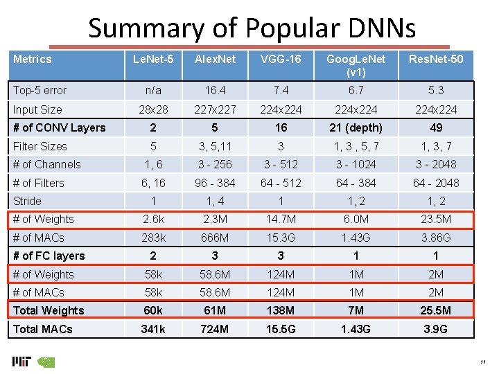
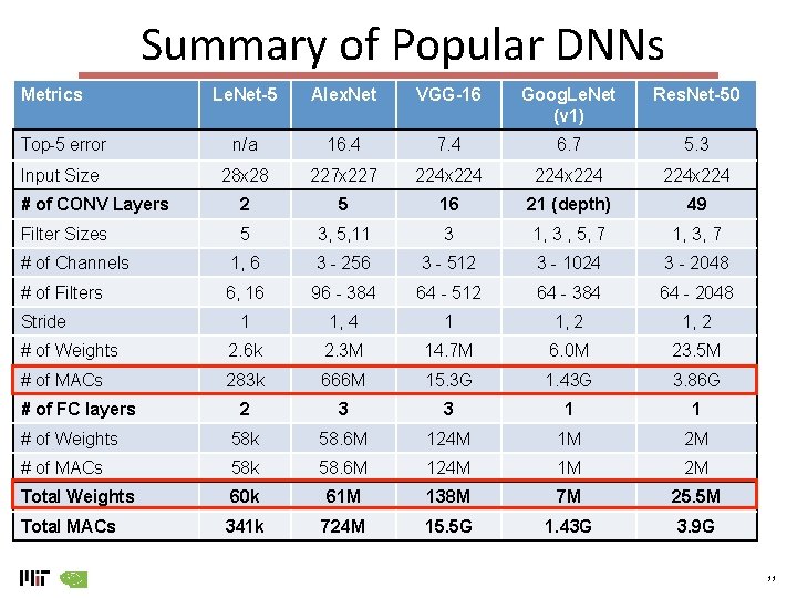
Summary of Popular DNNs Metrics Le. Net-5 Alex. Net VGG-16 Goog. Le. Net (v 1) Res. Net-50 Top-5 error n/a 16. 4 7. 4 6. 7 5. 3 Input Size 28 x 28 227 x 227 224 x 224 # of CONV Layers 2 5 16 21 (depth) 49 Filter Sizes 5 3, 5, 11 3 1, 3 , 5, 7 1, 3, 7 # of Channels 1, 6 3 - 256 3 - 512 3 - 1024 3 - 2048 # of Filters 6, 16 96 - 384 64 - 512 64 - 384 64 - 2048 1 1, 4 1 1, 2 # of Weights 2. 6 k 2. 3 M 14. 7 M 6. 0 M 23. 5 M # of MACs 283 k 666 M 15. 3 G 1. 43 G 3. 86 G 2 3 3 1 1 # of Weights 58 k 58. 6 M 124 M 1 M 2 M # of MACs 58 k 58. 6 M 124 M 1 M 2 M Total Weights 60 k 61 M 138 M 7 M 25. 5 M Total MACs 341 k 724 M 15. 5 G 1. 43 G 3. 9 G Stride # of FC layers 11

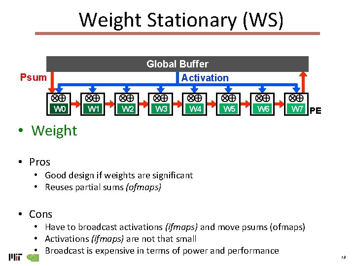
Weight Stationary (WS) Global Buffer Activation Psum W 0 W 1 W 2 W 3 W 4 W 5 W 6 W 7 PE • Weight • Pros • Good design if weights are significant • Reuses partial sums (ofmaps) • Cons • Have to broadcast activations (ifmaps) and move psums (ofmaps) • Activations (ifmaps) are not that small • Broadcast is expensive in terms of power and performance 18

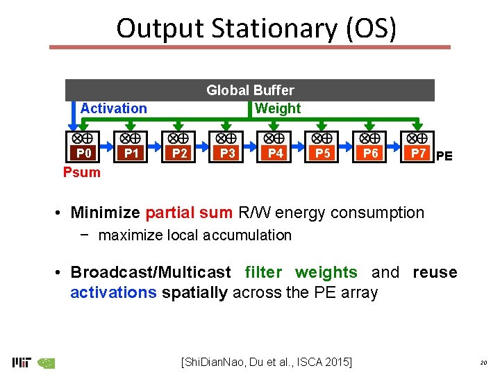
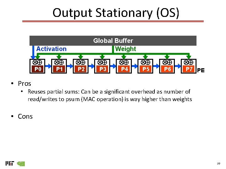
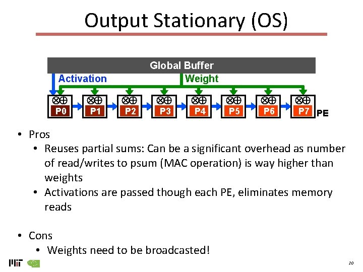
Output Stationary (OS) Global Buffer Weight Activation P 0 P 1 P 2 P 3 P 4 P 5 P 6 P 7 PE Psum • Minimize partial sum R/W energy consumption − maximize local accumulation • Broadcast/Multicast filter weights and reuse activations spatially across the PE array [Shi. Dian. Nao, Du et al. , ISCA 2015] 20

Output Stationary (OS) Global Buffer Weight Activation P 0 P 1 P 2 P 3 P 4 P 5 P 6 P 7 PE • Pros • Reuses partial sums: Can be a significant overhead as number of read/writes to psum (MAC operation) is way higher than weights • Cons 20

Summary of Popular DNNs Metrics Le. Net-5 Alex. Net VGG-16 Goog. Le. Net (v 1) Res. Net-50 Top-5 error n/a 16. 4 7. 4 6. 7 5. 3 Input Size 28 x 28 227 x 227 224 x 224 # of CONV Layers 2 5 16 21 (depth) 49 Filter Sizes 5 3, 5, 11 3 1, 3 , 5, 7 1, 3, 7 # of Channels 1, 6 3 - 256 3 - 512 3 - 1024 3 - 2048 # of Filters 6, 16 96 - 384 64 - 512 64 - 384 64 - 2048 1 1, 4 1 1, 2 # of Weights 2. 6 k 2. 3 M 14. 7 M 6. 0 M 23. 5 M # of MACs 283 k 666 M 15. 3 G 1. 43 G 3. 86 G 2 3 3 1 1 # of Weights 58 k 58. 6 M 124 M 1 M 2 M # of MACs 58 k 58. 6 M 124 M 1 M 2 M Total Weights 60 k 61 M 138 M 7 M 25. 5 M Total MACs 341 k 724 M 15. 5 G 1. 43 G 3. 9 G Stride # of FC layers 11

Output Stationary (OS) Global Buffer Weight Activation P 0 P 1 P 2 P 3 P 4 P 5 P 6 P 7 PE • Pros • Reuses partial sums: Can be a significant overhead as number of read/writes to psum (MAC operation) is way higher than weights • Activations are passed though each PE, eliminates memory reads • Cons • Weights need to be broadcasted! 20

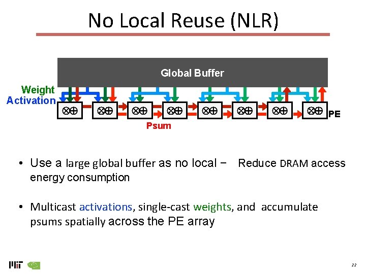
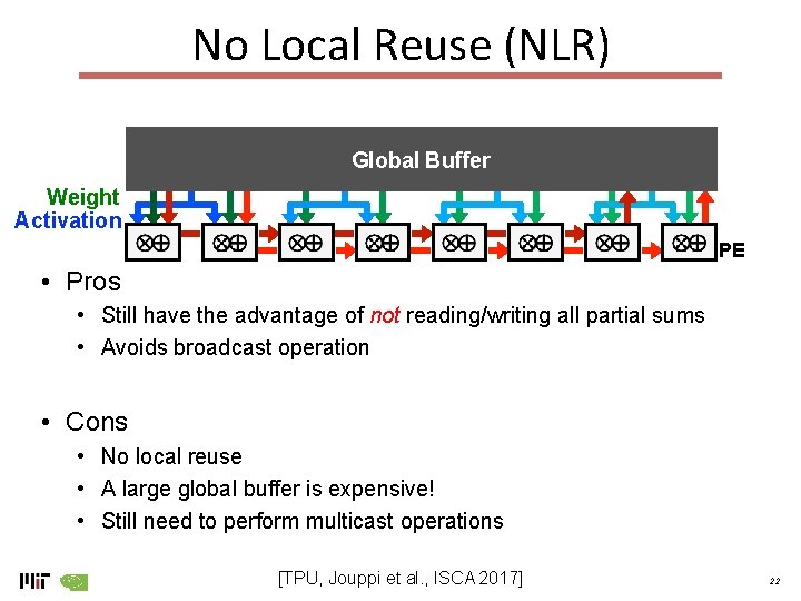
No Local Reuse (NLR) • Psum Global Buffer Weight Activation PE Psum • Use a large global buffer as no local − Reduce DRAM access energy consumption • Multicast activations, single-cast weights, and accumulate psums spatially across the PE array 22

No Local Reuse (NLR) • Psum Global Buffer Weight Activation PE • Pros • Still have the advantage of not reading/writing all partial sums • Avoids broadcast operation • Cons • No local reuse • A large global buffer is expensive! • Still need to perform multicast operations [TPU, Jouppi et al. , ISCA 2017] 22

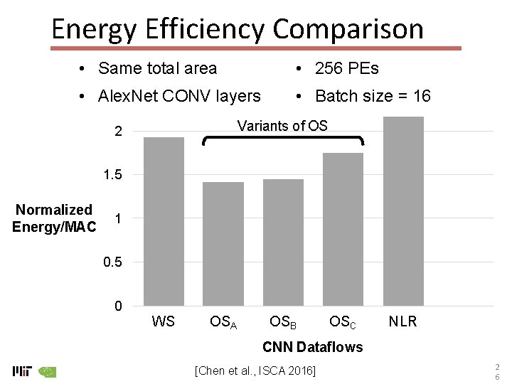
Energy Efficiency Comparison • Same total area • 256 PEs • Alex. Net CONV layers • Batch size = 16 Variants of OS 2 1. 5 Normalized Energy/MAC 1 0. 5 0 WS OSA OSB OSC NLR CNN Dataflows [Chen et al. , ISCA 2016] 2 6

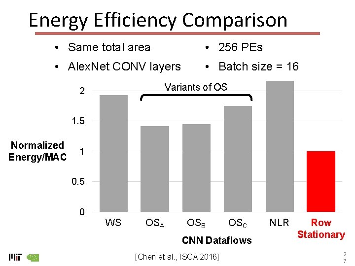
Energy Efficiency Comparison • Same total area • 256 PEs • Alex. Net CONV layers • Batch size = 16 Variants of OS 2 1. 5 Normalized Energy/MAC 1 0. 5 0 WS OSA OSB OSC CNN Dataflows [Chen et al. , ISCA 2016] NLR Row Stationary 2 7

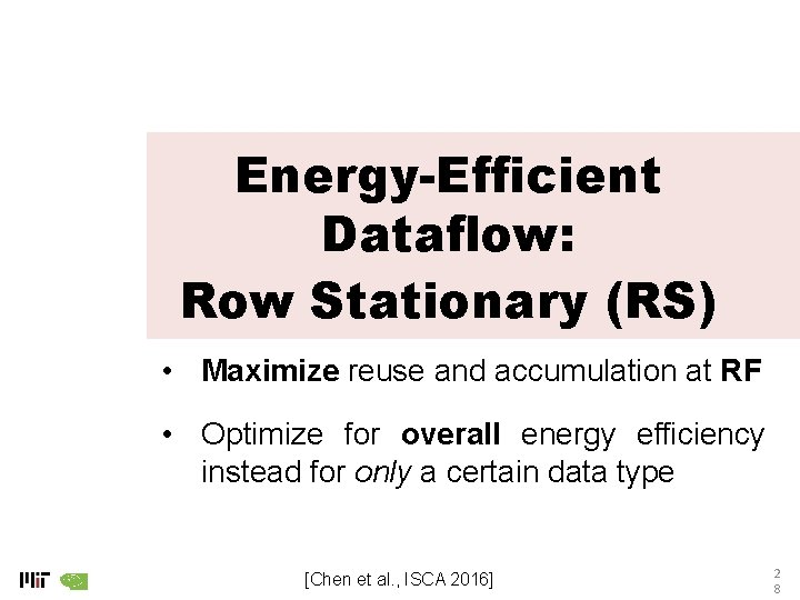
Energy-Efficient Dataflow: Row Stationary (RS) • Maximize reuse and accumulation at RF • Optimize for overall energy efficiency instead for only a certain data type [Chen et al. , ISCA 2016] 2 8

Summary of Popular DNNs Metrics Le. Net-5 Alex. Net VGG-16 Goog. Le. Net (v 1) Res. Net-50 Top-5 error n/a 16. 4 7. 4 6. 7 5. 3 Input Size 28 x 28 227 x 227 224 x 224 # of CONV Layers 2 5 16 21 (depth) 49 Filter Sizes 5 3, 5, 11 3 1, 3 , 5, 7 1, 3, 7 # of Channels 1, 6 3 - 256 3 - 512 3 - 1024 3 - 2048 # of Filters 6, 16 96 - 384 64 - 512 64 - 384 64 - 2048 1 1, 4 1 1, 2 # of Weights 2. 6 k 2. 3 M 14. 7 M 6. 0 M 23. 5 M # of MACs 283 k 666 M 15. 3 G 1. 43 G 3. 86 G 2 3 3 1 1 # of Weights 58 k 58. 6 M 124 M 1 M 2 M # of MACs 58 k 58. 6 M 124 M 1 M 2 M Total Weights 60 k 61 M 138 M 7 M 25. 5 M Total MACs 341 k 724 M 15. 5 G 1. 43 G 3. 9 G Stride # of FC layers 11

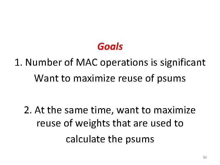
Goals 1. Number of MAC operations is significant Want to maximize reuse of psums 2. At the same time, want to maximize reuse of weights that are used to calculate the psums 50

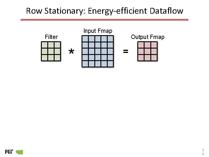
Row Stationary: Energy-efficient Dataflow Input Fmap Filter * Output Fmap = 2 9

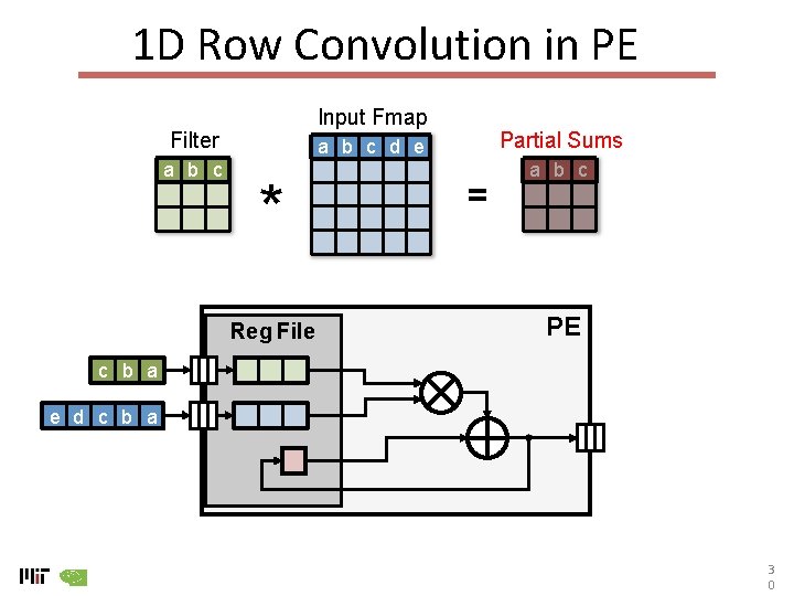
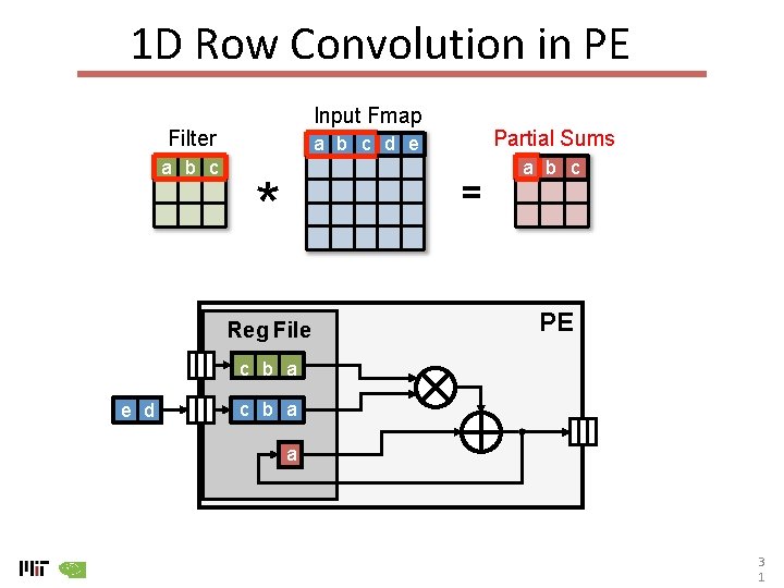
1 D Row Convolution in PE Input Fmap Filter a b c Partial Sums a b c d e * Reg File = a b c PE c b a e d c b a 3 0

1 D Row Convolution in PE Input Fmap Filter a b c Partial Sums a b c d e * = Reg File a b c PE c b a e d c b a a 3 1

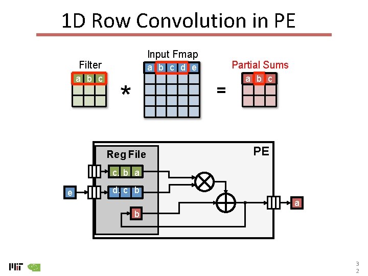
1 D Row Convolution in PE Input Fmap Filter a b c Partial Sums a b c d e * = Reg File a b c PE c. b a e d. c b a b 3 2

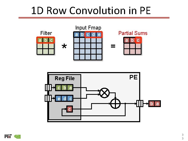
1 D Row Convolution in PE Input Fmap Filter a b c Partial Sums a b c d e * = Reg File a b c PE c b a e d c b a c 3 3

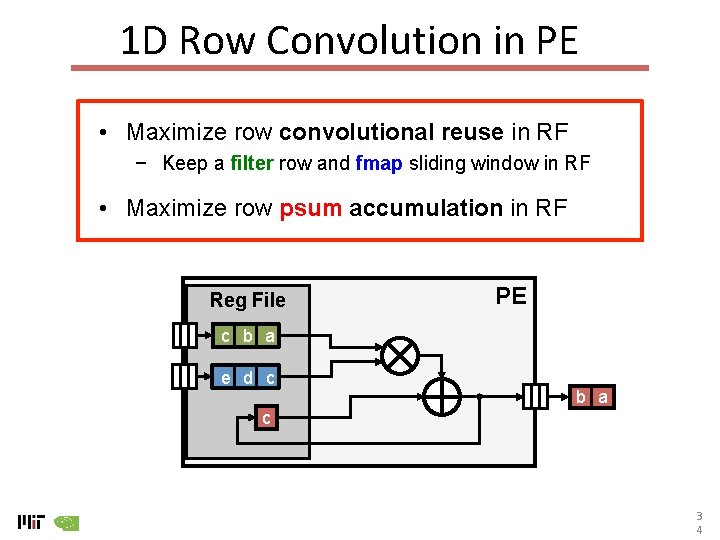
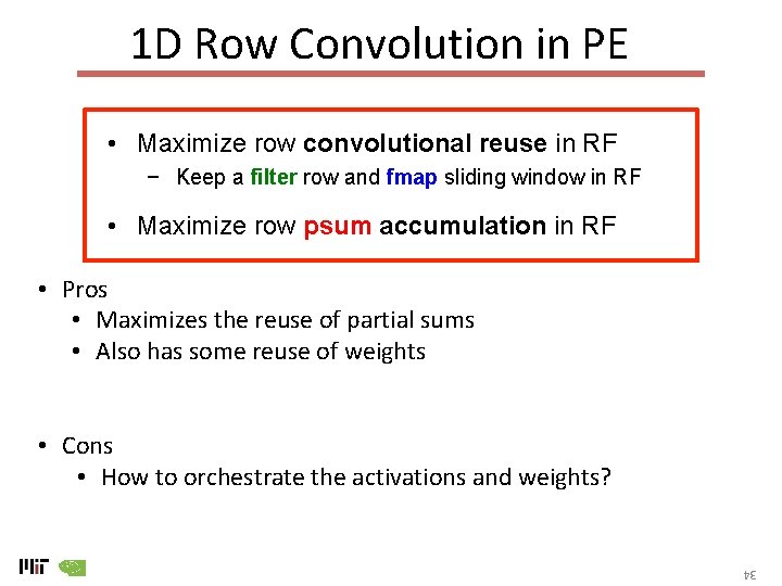
1 D Row Convolution in PE • Maximize row convolutional reuse in RF − Keep a filter row and fmap sliding window in RF • Maximize row psum accumulation in RF Reg File PE c b a e d c b a c 3 4

1 D Row Convolution in PE • Maximize row convolutional reuse in RF − Keep a filter row and fmap sliding window in RF • Maximize row psum accumulation in RF • Pros • Maximizes the reuse of partial sums • Also has some reuse of weights • Cons • How to orchestrate the activations and weights? 34

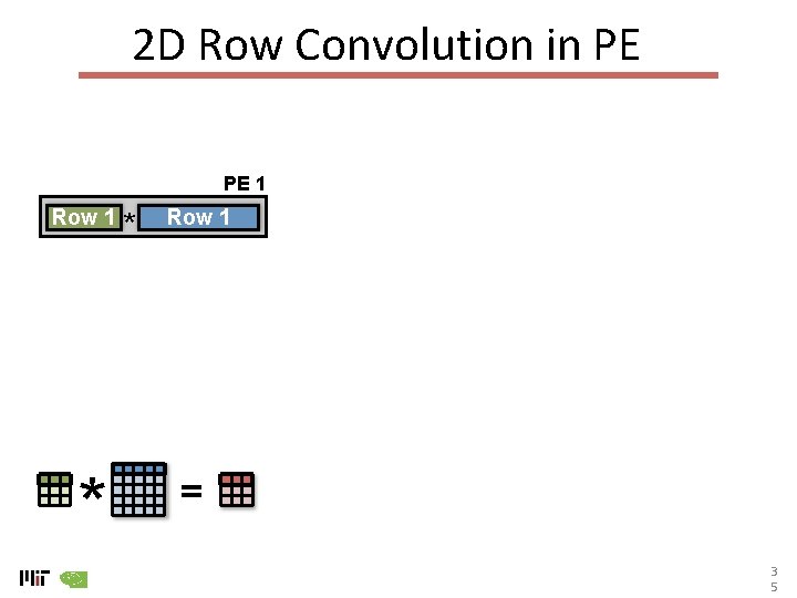
2 D Row Convolution in PE PE 1 Row 1 * * Row 1 = 3 5

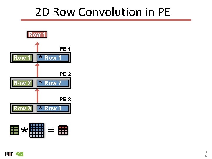
2 D Row Convolution in PE Row 1 PE 1 Row 1 * Row 1 PE 2 Row 2 * Row 2 PE 3 Row 3 * * Row 3 = 3 6

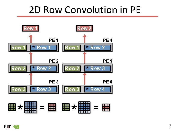
2 D Row Convolution in PE Row 1 Row 2 PE 1 Row 1 * Row 1 PE 4 Row 1 * Row 2 PE 2 Row 2 * Row 2 PE 5 Row 2 * Row 3 PE 3 Row 3 * * Row 3 = PE 6 Row 3 * * Row 4 = 3 7

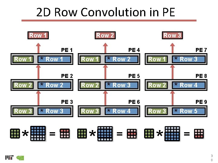
2 D Row Convolution in PE Row 1 Row 2 Row 3 PE 1 Row 1 * Row 1 PE 4 Row 1 * Row 2 PE 2 Row 2 * * Row 3 = Row 1 * Row 3 PE 5 Row 2 * Row 3 PE 3 Row 3 PE 7 PE 8 Row 2 * Row 4 PE 6 Row 3 * * Row 4 = PE 9 Row 3 * * Row 5 = 3 8

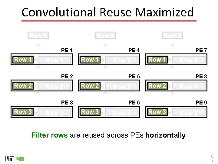
Convolutional Reuse Maximized Row 1 Row 2 PE 1 Row 1 * Row 1 PE 4 Row 1 * PE 2 Row 2 * Row 3 Row 2 PE 7 Row 1 * Row 3 PE 5 Row 2 * PE 3 Row 3 PE 8 Row 2 * Row 4 PE 6 Row 3 * Row 4 PE 9 Row 3 * Row 5 Filter rows are reused across PEs horizontally 3 9

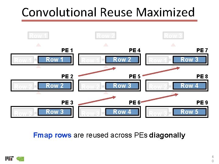
Convolutional Reuse Maximized Row 1 Row 2 PE 1 Row 1 * Row 1 PE 4 Row 1 * PE 2 Row 2 * Row 3 Row 2 PE 7 Row 1 * Row 3 PE 5 Row 2 * PE 3 Row 3 PE 8 Row 2 * Row 4 PE 6 Row 3 * Row 4 PE 9 Row 3 * Row 5 Fmap rows are reused across PEs diagonally 4 0

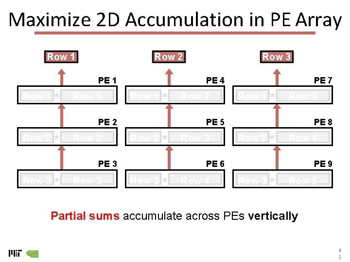
Maximize 2 D Accumulation in PE Array Row 1 Row 2 PE 1 Row 1 * Row 1 PE 4 Row 1 * PE 2 Row 2 * Row 3 Row 2 PE 7 Row 1 * Row 3 PE 5 Row 2 * PE 3 Row 3 PE 8 Row 2 * Row 4 PE 6 Row 3 * Row 4 PE 9 Row 3 * Row 5 Partial sums accumulate across PEs vertically 4 1

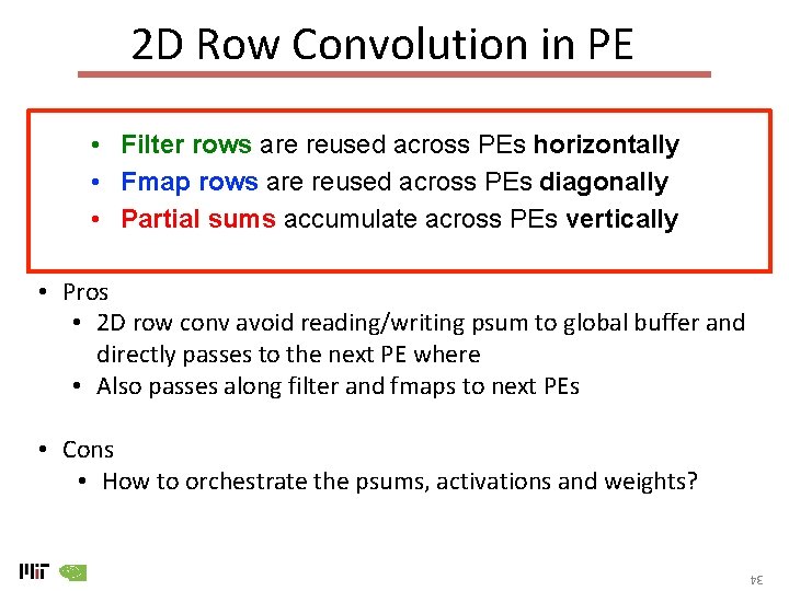
2 D Row Convolution in PE • Filter rows are reused across PEs horizontally • Fmap rows are reused across PEs diagonally • Partial sums accumulate across PEs vertically • Pros • 2 D row conv avoid reading/writing psum to global buffer and directly passes to the next PE where • Also passes along filter and fmaps to next PEs • Cons • How to orchestrate the psums, activations and weights? 34

Dimensions Beyond 2 D Convolution 1 Multiple Fmaps 2 Multiple Filters 3 Multiple Channels 4 2

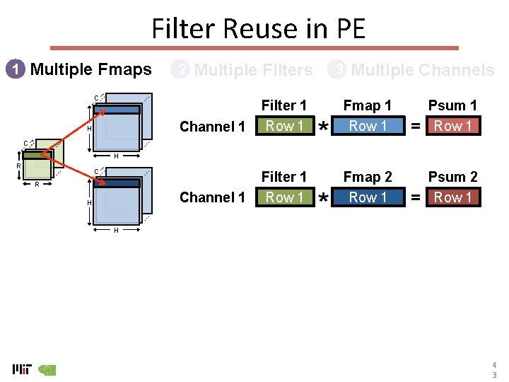
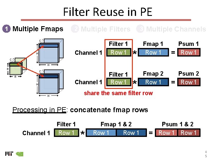
Filter Reuse in PE Multiple Fmaps 1 2 Multiple Filters C H Channel 1 Filter 1 Row 1 C 3 * Multiple Channels Fmap 1 Row 1 = Psum 2 Row 1 H R C R H * Fmap 2 Row 1 H 4 3

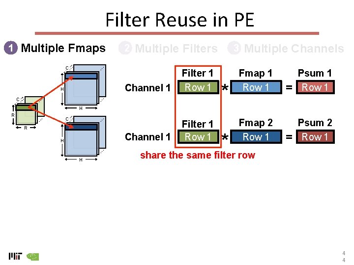
Filter Reuse in PE Multiple Fmaps 1 2 Multiple Filters C Channel 1 H Filter 1 Row 1 C 3 * Multiple Channels Fmap 1 Row 1 = Psum 2 Row 1 H R C R H Fmap 2 Row 1 * share the same filter row Channel 1 H Filter 1 Row 1 4 4

Filter Reuse in PE Multiple Fmaps 1 2 Multiple Filters C Channel 1 H Filter 1 Row 1 C 3 * Multiple Channels Fmap 1 Row 1 = Psum 2 Row 1 H R C R Fmap 2 Row 1 * share the same filter row Channel 1 H Filter 1 Row 1 H Processing in PE: concatenate fmap rows Channel 1 Filter 1 Row 1 * Fmap 1 & 2 Row 1 = Psum 1 & 2 Row 1 4 5

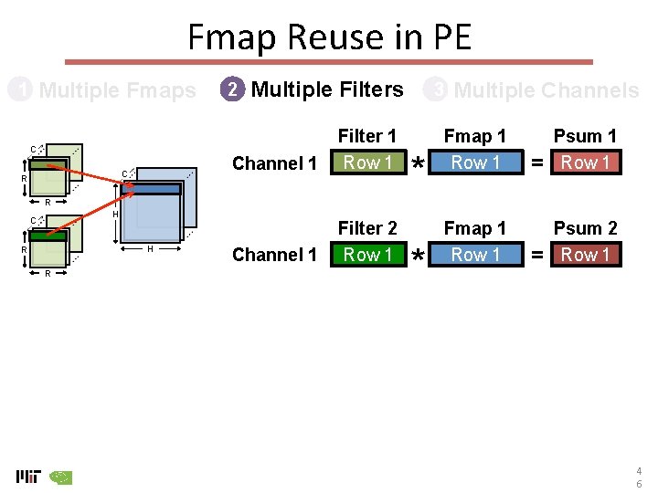
Fmap Reuse in PE Multiple Fmaps 1 C C R 2 Multiple Filters Channel 1 Filter 1 Row 1 Channel 1 Filter 2 Row 1 3 * Multiple Channels Fmap 1 Row 1 = Psum 2 Row 1 R H C H R R * Fmap 1 Row 1 4 6

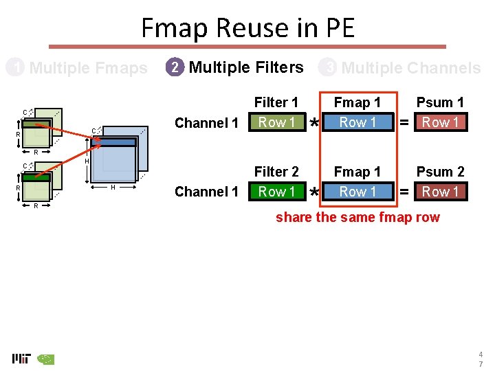
Fmap Reuse in PE Multiple Fmaps 1 C C R 2 Multiple Filters Channel 1 Filter 1 Row 1 Channel 1 Filter 2 Row 1 3 * Multiple Channels Fmap 1 Row 1 = Psum 1 Row 1 R H C H R R Fmap 1 Row 1 Psum 2 Row 1 * share the same fmap row = 4 7

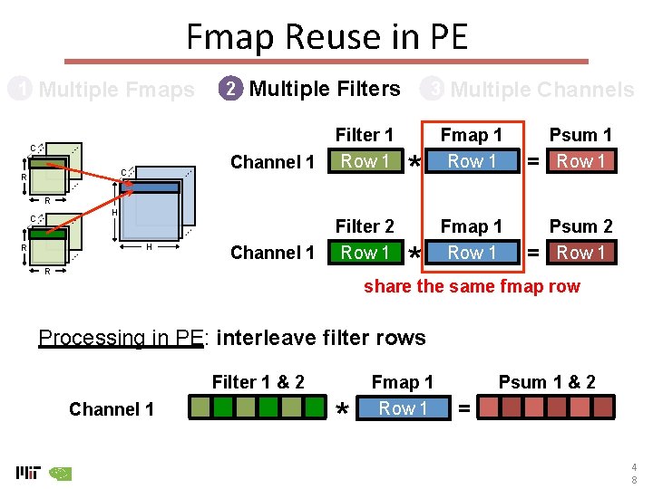
Fmap Reuse in PE Multiple Fmaps 1 C C R 2 Multiple Filters Channel 1 Filter 1 Row 1 Channel 1 Filter 2 Row 1 3 * Multiple Channels Fmap 1 Row 1 = Psum 1 Row 1 R H C H R Fmap 1 Row 1 Psum 2 Row 1 * share the same fmap row R = Processing in PE: interleave filter rows Filter 1 & 2 Channel 1 * Fmap 1 Row 1 Psum 1 & 2 = 4 8

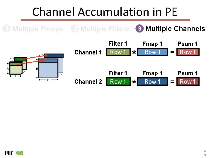
Channel Accumulation in PE Multiple Fmaps 1 C 2 Multiple Filters Channel 1 Filter 1 Row 1 Channel 2 Filter 1 Row 1 C H R R H 3 * * Multiple Channels Fmap 1 Row 1 = Psum 1 Row 1 4 9

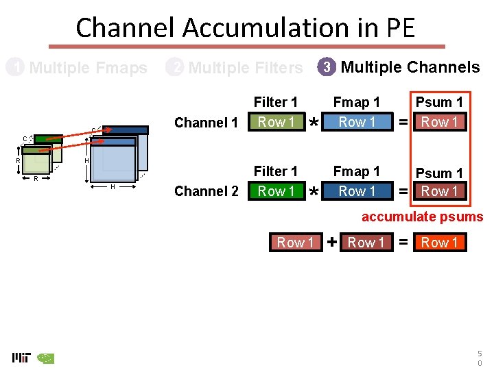
Channel Accumulation in PE Multiple Fmaps 1 C 2 Multiple Filters Channel 1 Filter 1 Row 1 Channel 2 Filter 1 Row 1 C H R R H Multiple Channels 3 * * Row 1 Fmap 1 Row 1 = Psum 1 Row 1 accumulate psums + Row 1 = Row 1 5 0

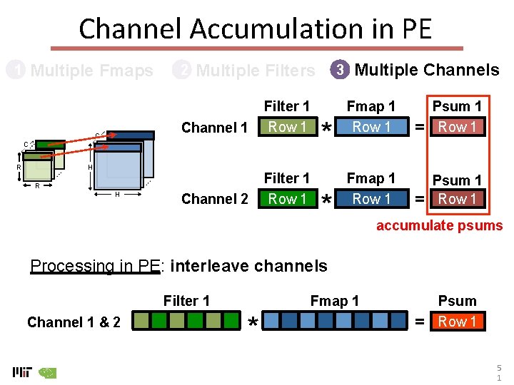
Channel Accumulation in PE Multiple Fmaps 1 C 2 Multiple Filters Channel 1 Filter 1 Row 1 Channel 2 Filter 1 Row 1 C H R R H 3 * * Multiple Channels Fmap 1 Row 1 = Psum 1 Row 1 accumulate psums Processing in PE: interleave channels Filter 1 Channel 1 & 2 Fmap 1 * = Psum Row 1 5 1

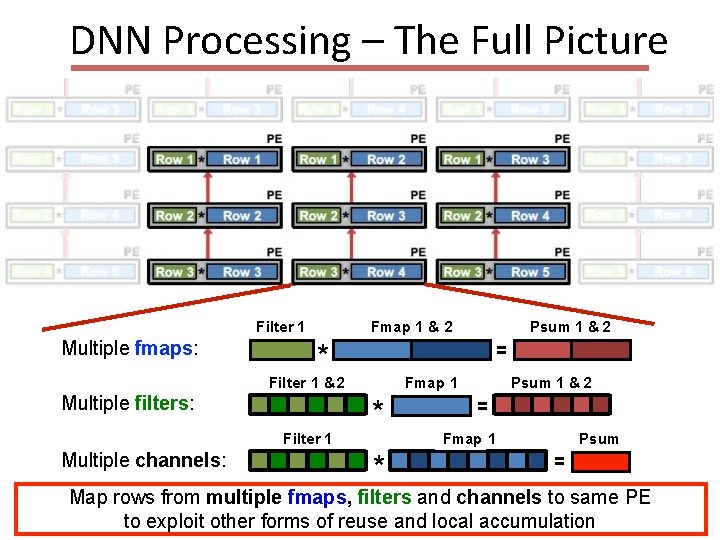
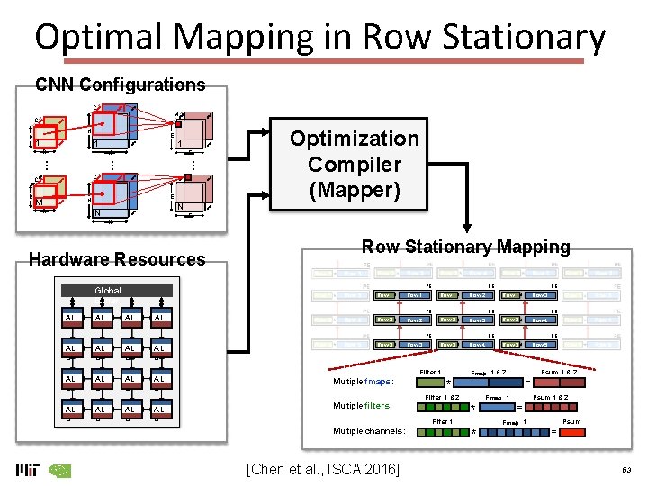
DNN Processing – The Full Picture Filter 1 Multiple fmaps: * = Filter 1 & 2 Multiple filters: Filter 1 Multiple channels: Psum 1 & 2 Image Fmap 1 & 2 Psum 1 & 2 Image Fmap 1 * * = Fmap 1 Image Psum = Map rows from multiple fmaps, filters and channels to same PE to exploit other forms of reuse and local accumulation 52

Optimal Mapping in Row Stationary CNN Configurations C M C H 1 E 1 1 R H … … C C R E … R M E H R N N E H Hardware Resources AL U Row Stationary Mapping PE Global Buffer AL U Optimization Compiler (Mapper) AL U Row 1 * Row 1 Row 2 * Row 2 Row 3 * Row 3 PE Row 1 * Row 2 * Row 3 * Row 4 PE AL U AL U AL U * Multiple filters: Filter 1 Multiple channels: [Chen et al. , ISCA 2016] Row 4 Row 3 * Row 5 PE PE Image Fmap 1 & 2 Psum 1 & 2 = Filter 1 & 2 AL U Row 2 * PE Filter 1 Multiple fmaps: Row 3 PE PE AL U PE Row 1 * Image Fmap 1 * * Psum 1 & 2 = Image Fmap 1 Psum = 53

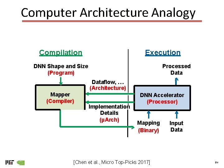
Computer Architecture Analogy Compilation Execution DNN Shape and Size (Program) Processed Dataflow, … (Architecture) Mapper (Compiler) Implementation Details (µArch) DNN Accelerator (Processor) Mapping (Binary) [Chen et al. , Micro Top-Picks 2017] Input Data 54

ADVANCED COMPUTER ARCHITECTURE ML Accelerators Samira Khan University of Virginia Feb 6, 2019 The content and concept of this course are adapted from CMU ECE 740