ADVANCED COMPUTER ARCHITECTURE ML Accelerators Why Samira Khan

ADVANCED COMPUTER ARCHITECTURE ML Accelerators: Why Samira Khan University of Virginia Feb 4, 2019 The content and concept of this course are adapted from CMU ECE 740

AGENDA • Review from last lecture • Single core->multi core->accelerator • ML accelerators: why? 2

LOGISTICS • Project list – Posted in Piazza – Be prepared to spend time on the project • Sample project proposals from many different years – Posted in Piazza • Project Proposal Due on Feb 11, 2019 • Project Proposal Presentations: Feb 13, 2019 – Can can present using your own laptop • Groups: 1 or 2 students 3

Project Proposal • Problem: Clearly define what is the problem you are trying to solve • Novelty: Did any other work try to solve the problem? How did they solve it? What are the shortcomings? • Key Idea: What is the initial idea? Why do you think it will work? How is your approach different from the prior work? • Methodology: How will you test and evaluate your idea? What tools or simulators will you use? What are the experiments you need to do to prove/disprove your idea? • Plan: Describe the steps to finish your project. What will you accomplice at each milestone? What are things you must need to finish? Can you do more? If you finish it can you submit it to a conference? Which conference do you think is a better fit for the work? 4

LITERATURE SURVEY • Goal: Critically analyze related work to your project • Pick 2 -3 papers related to your project • Use the same format as the reviews – What is the problem the paper is solving – What is the key insight – What are the advantages and disadvantages – How can you do better • Will become the related work in your proposal 5

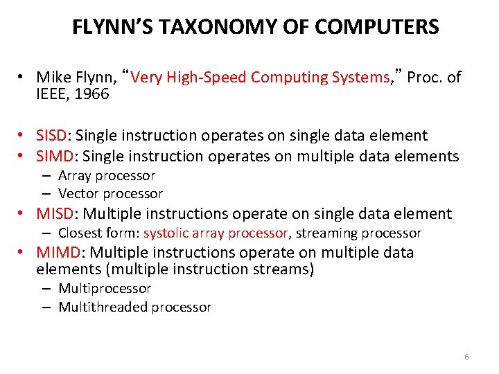
FLYNN’S TAXONOMY OF COMPUTERS • Mike Flynn, “Very High-Speed Computing Systems, ” Proc. of IEEE, 1966 • SISD: Single instruction operates on single data element • SIMD: Single instruction operates on multiple data elements – Array processor – Vector processor • MISD: Multiple instructions operate on single data element – Closest form: systolic array processor, streaming processor • MIMD: Multiple instructions operate on multiple data elements (multiple instruction streams) – Multiprocessor – Multithreaded processor 6

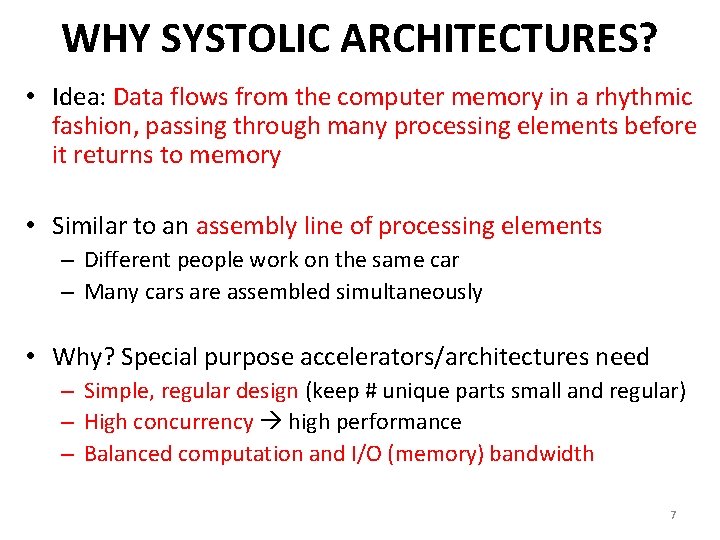
WHY SYSTOLIC ARCHITECTURES? • Idea: Data flows from the computer memory in a rhythmic fashion, passing through many processing elements before it returns to memory • Similar to an assembly line of processing elements – Different people work on the same car – Many cars are assembled simultaneously • Why? Special purpose accelerators/architectures need – Simple, regular design (keep # unique parts small and regular) – High concurrency high performance – Balanced computation and I/O (memory) bandwidth 7

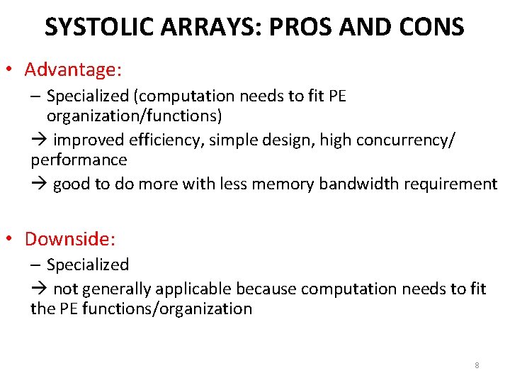
SYSTOLIC ARRAYS: PROS AND CONS • Advantage: – Specialized (computation needs to fit PE organization/functions) improved efficiency, simple design, high concurrency/ performance good to do more with less memory bandwidth requirement • Downside: – Specialized not generally applicable because computation needs to fit the PE functions/organization 8

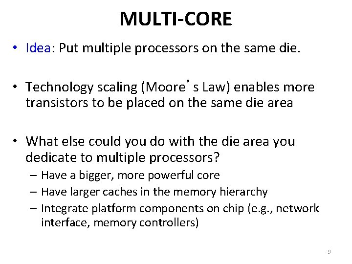
MULTI-CORE • Idea: Put multiple processors on the same die. • Technology scaling (Moore’s Law) enables more transistors to be placed on the same die area • What else could you do with the die area you dedicate to multiple processors? – Have a bigger, more powerful core – Have larger caches in the memory hierarchy – Integrate platform components on chip (e. g. , network interface, memory controllers) 9

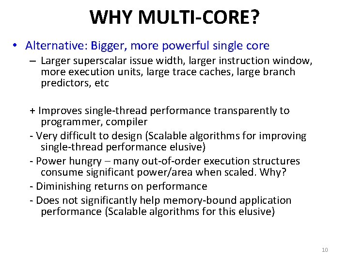
WHY MULTI-CORE? • Alternative: Bigger, more powerful single core – Larger superscalar issue width, larger instruction window, more execution units, large trace caches, large branch predictors, etc + Improves single-thread performance transparently to programmer, compiler - Very difficult to design (Scalable algorithms for improving single-thread performance elusive) - Power hungry – many out-of-order execution structures consume significant power/area when scaled. Why? - Diminishing returns on performance - Does not significantly help memory-bound application performance (Scalable algorithms for this elusive) 10

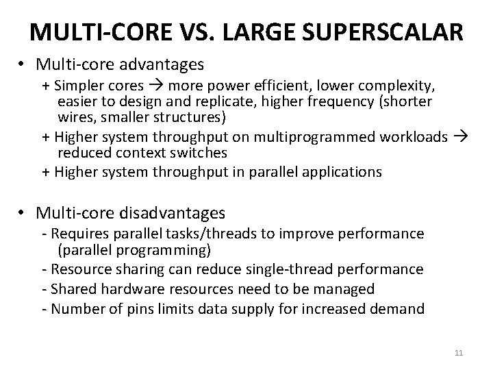
MULTI-CORE VS. LARGE SUPERSCALAR • Multi-core advantages + Simpler cores more power efficient, lower complexity, easier to design and replicate, higher frequency (shorter wires, smaller structures) + Higher system throughput on multiprogrammed workloads reduced context switches + Higher system throughput in parallel applications • Multi-core disadvantages - Requires parallel tasks/threads to improve performance (parallel programming) - Resource sharing can reduce single-thread performance - Shared hardware resources need to be managed - Number of pins limits data supply for increased demand 11

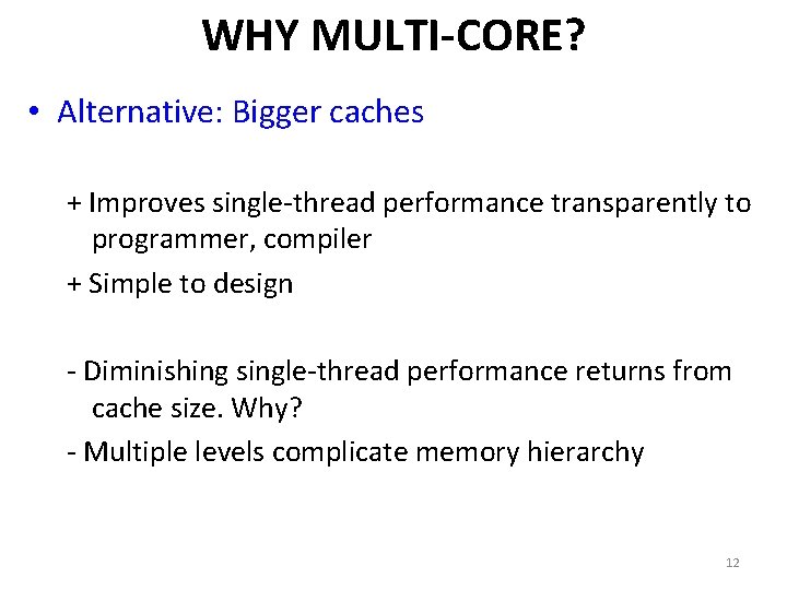
WHY MULTI-CORE? • Alternative: Bigger caches + Improves single-thread performance transparently to programmer, compiler + Simple to design - Diminishing single-thread performance returns from cache size. Why? - Multiple levels complicate memory hierarchy 12

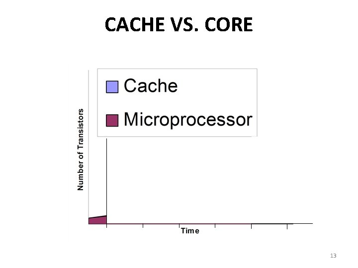
CACHE VS. CORE 13

WHY MULTI-CORE? • Alternative: Integrate platform components on chip instead + Speeds up many system functions (e. g. , network interface cards, Ethernet controller, memory controller, I/O controller) - Not all applications benefit (e. g. , CPU intensive code sections) 14

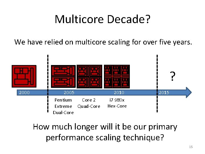
Multicore Decade? We have relied on multicore scaling for over five years. ? 2000 2005 Pentium Core 2 Extreme Quad-Core Dual-Core 2010 i 7 980 x Hex-Core 2015 How much longer will it be our primary performance scaling technique? 15

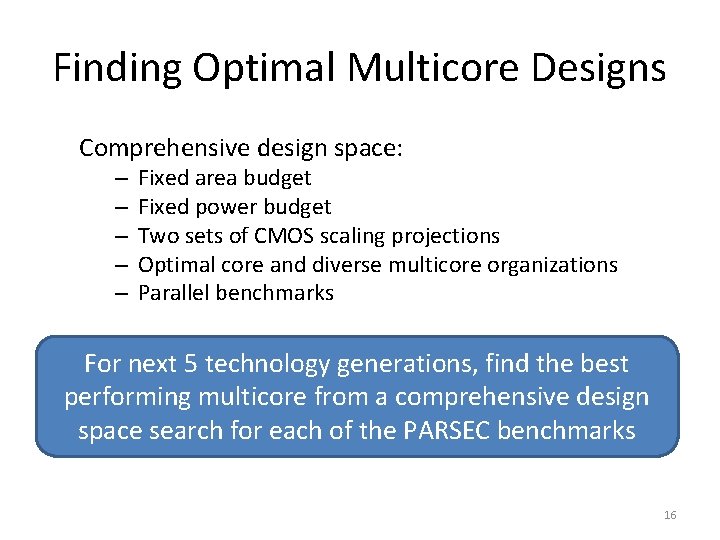
Finding Optimal Multicore Designs Comprehensive design space: – – – Fixed area budget Fixed power budget Two sets of CMOS scaling projections Optimal core and diverse multicore organizations Parallel benchmarks For next 5 technology generations, find the best performing multicore from a comprehensive design space search for each of the PARSEC benchmarks 16

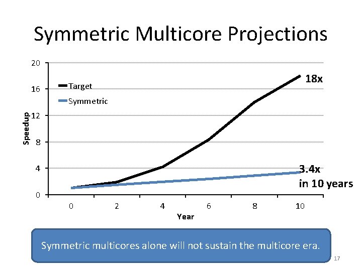
Symmetric Multicore Projections 20 16 18 x Target Speedup Symmetric 12 8 3. 4 x in 10 years 4 0 0 2 4 Year 6 8 10 Symmetric multicores alone will not sustain the multicore era. 17

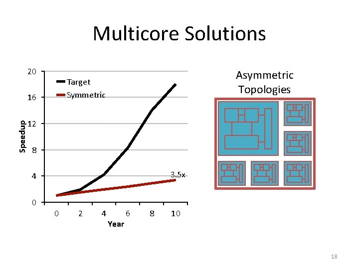
Multicore Solutions 20 Asymmetric Topologies Target Symmetric 16 Speedup Asymmetric 12 8 3. 5 x 4 0 0 2 4 Year 6 8 10 18

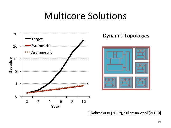
Multicore Solutions 20 Dynamic Topologies Target Symmetric 16 Speedup Asymmetric 12 Dynamic 8 3. 5 x 4 0 0 2 4 Year 6 8 10 [Chakraborty (2008), Suleman et al (2009)] 19

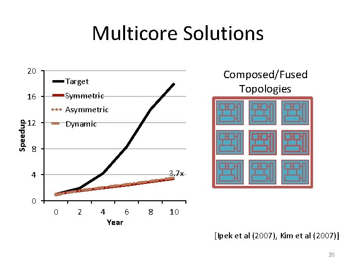
Multicore Solutions Speedup 20 Composed/Fused Topologies Target 16 Symmetric Asymmetric 12 Dynamic Composed 8 3. 7 x 4 0 0 2 4 Year 6 8 10 [Ipek et al (2007), Kim et al (2007)] 20

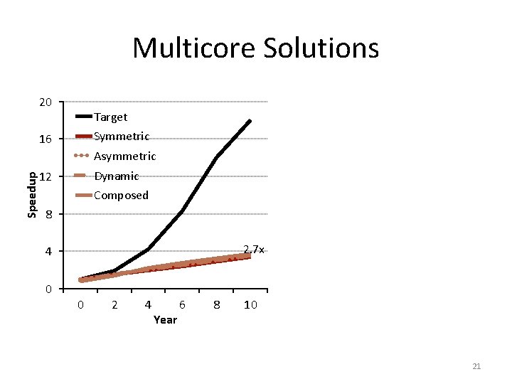
Multicore Solutions 20 Target Symmetric 16 Speedup Asymmetric Dynamic 12 Composed 8 GPU 2. 7 x 4 0 0 2 4 Year 6 8 10 21

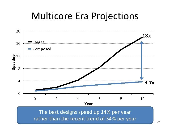
Multicore Era Projections 20 16 18 x Target Speedup Composed 12 8 4 0 3. 7 x 0 2 4 Year 6 8 The best designs speed up 14% per year rather than the recent trend of 34% per year 10 22

WITH MULTIPLE CORES ON CHIP • What we want: – N times the performance with N times the cores when we parallelize an application on N cores • What we get: – Amdahl’s Law (serial bottleneck) – Bottlenecks in the parallel portion 23

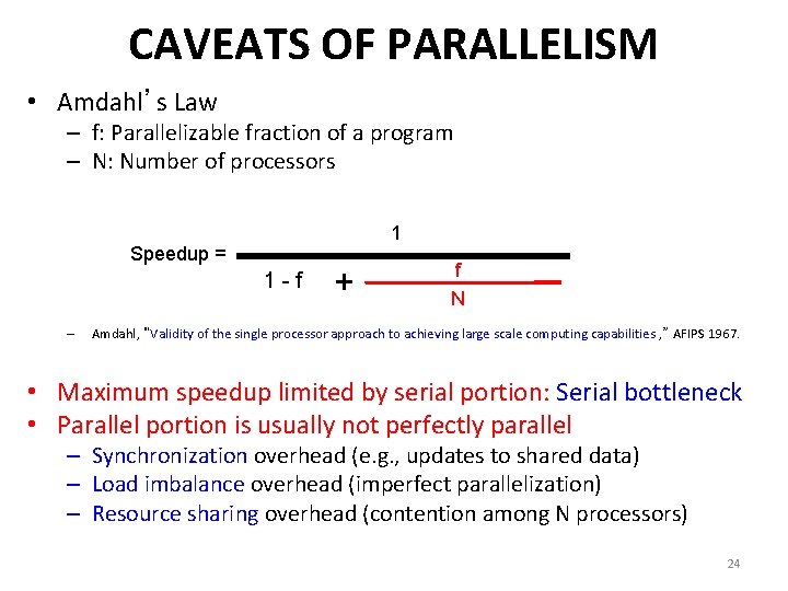
CAVEATS OF PARALLELISM • Amdahl’s Law – f: Parallelizable fraction of a program – N: Number of processors 1 Speedup = 1 -f – + f N Amdahl, “Validity of the single processor approach to achieving large scale computing capabilities , ” AFIPS 1967. • Maximum speedup limited by serial portion: Serial bottleneck • Parallel portion is usually not perfectly parallel – Synchronization overhead (e. g. , updates to shared data) – Load imbalance overhead (imperfect parallelization) – Resource sharing overhead (contention among N processors) 24

THE PROBLEM: SERIALIZED CODE SECTIONS • Many parallel programs cannot be parallelized completely • Causes of serialized code sections – Sequential portions (Amdahl’s “serial part”) – Critical sections – Barriers • Serialized code sections – Reduce performance – Limit scalability – Waste energy 25

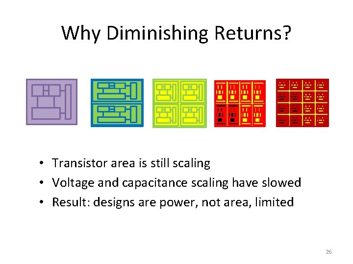
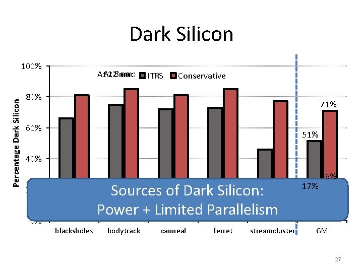
Why Diminishing Returns? • Transistor area is still scaling • Voltage and capacitance scaling have slowed • Result: designs are power, not area, limited 26

Dark Silicon Percentage Dark Silicon 100% At 8 nm: At 22 nm: ITRS Conservative 80% 71% 60% 51% 40% Sources of Dark Silicon: Power + Limited Parallelism 20% 0% blacksholes bodytrack canneal ferret streamcluster 17% 26% GM GM 27

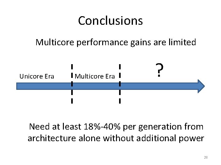
Conclusions Multicore performance gains are limited Unicore Era Multicore Era ? Need at least 18%-40% per generation from architecture alone without additional power 28

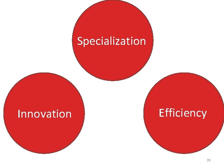
Specialization Innovation Efficiency 29

NN Accelerators 30

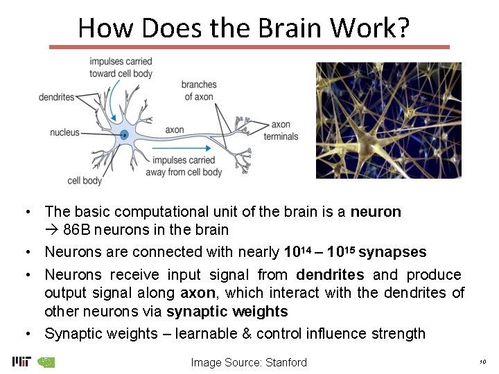
How Does the Brain Work? • The basic computational unit of the brain is a neuron 86 B neurons in the brain • Neurons are connected with nearly 1014 – 1015 synapses • Neurons receive input signal from dendrites and produce output signal along axon, which interact with the dendrites of other neurons via synaptic weights • Synaptic weights – learnable & control influence strength Image Source: Stanford 10

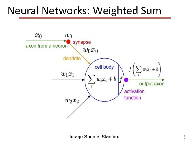
Neural Networks: Weighted Sum Image Source: Stanford 3 2

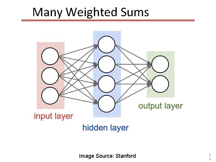
Many Weighted Sums Image Source: Stanford 3 3

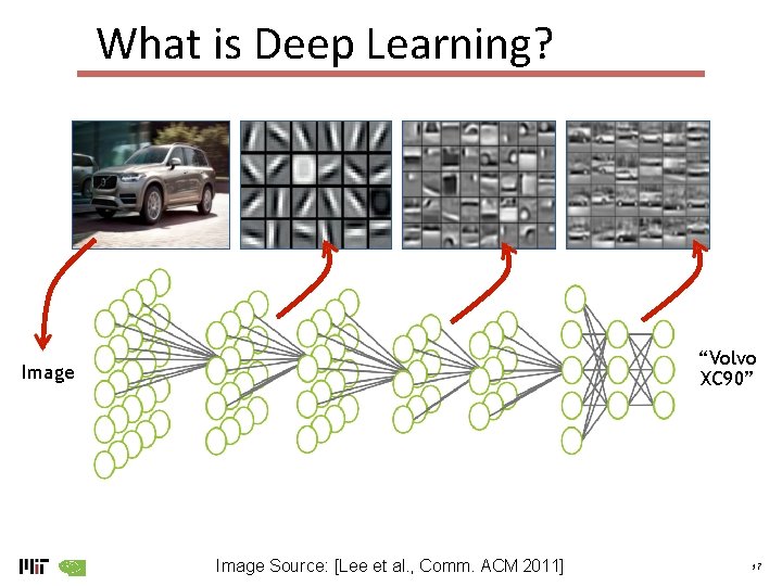
What is Deep Learning? “Volvo XC 90” Image Source: [Lee et al. , Comm. ACM 2011] 17

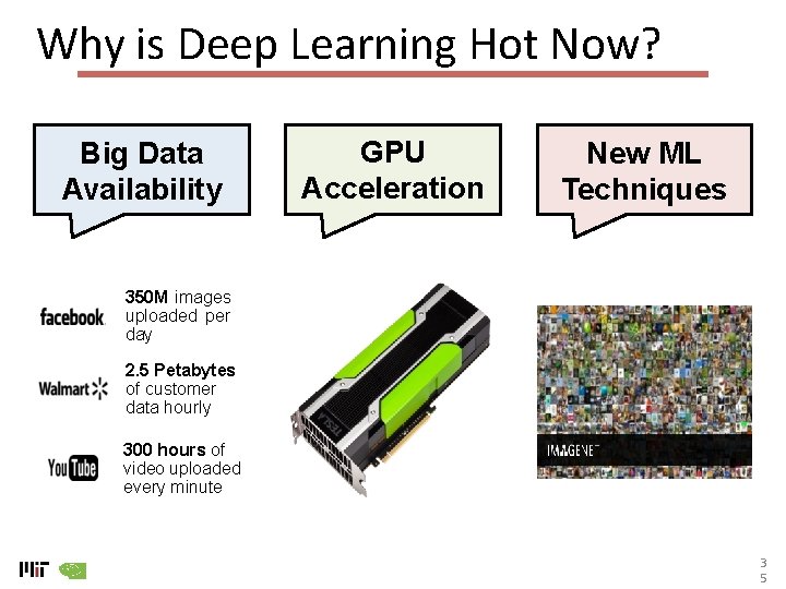
Why is Deep Learning Hot Now? Big Data Availability GPU Acceleration New ML Techniques 350 M images uploaded per day 2. 5 Petabytes of customer data hourly 300 hours of video uploaded every minute 3 5

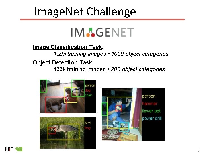
Image. Net Challenge Image Classification Task: 1. 2 M training images • 1000 object categories Object Detection Task: 456 k training images • 200 object categories 3 6

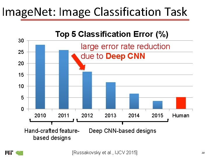
Image. Net: Image Classification Task Top 5 Classification Error (%) 30 large error rate reduction due to Deep CNN 25 20 15 10 5 0 2011 2012 Hand-crafted featurebased designs 2013 2014 2015 Human Deep CNN-based designs [Russakovsky et al. , IJCV 2015] 20

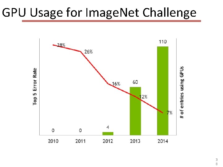
GPU Usage for Image. Net Challenge 3 8

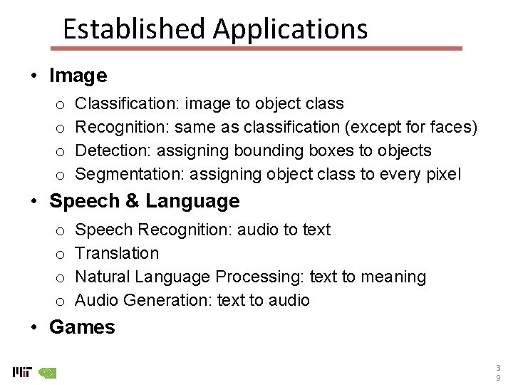
Established Applications • Image o o Classification: image to object class Recognition: same as classification (except for faces) Detection: assigning bounding boxes to objects Segmentation: assigning object class to every pixel • Speech & Language o o Speech Recognition: audio to text Translation Natural Language Processing: text to meaning Audio Generation: text to audio • Games 3 9

Deep Learning on Games Google Deep. Mind Alpha. Go

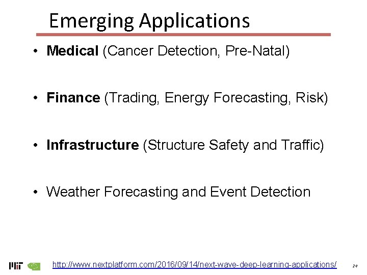
Emerging Applications • Medical (Cancer Detection, Pre-Natal) • Finance (Trading, Energy Forecasting, Risk) • Infrastructure (Structure Safety and Traffic) • Weather Forecasting and Event Detection http: //www. nextplatform. com/2016/09/14/next-wave-deep-learning-applications/ 24

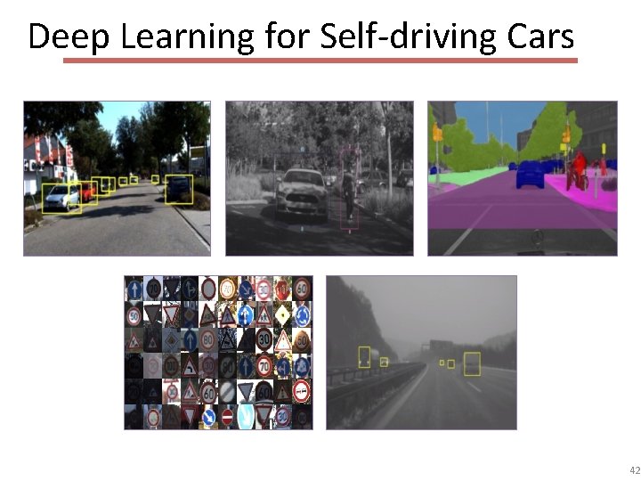
Deep Learning for Self-driving Cars 42

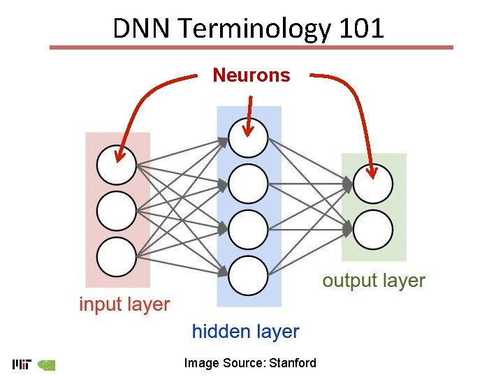
DNN Terminology 101 Neurons DNN Terminology 101 Image Source: Stanford

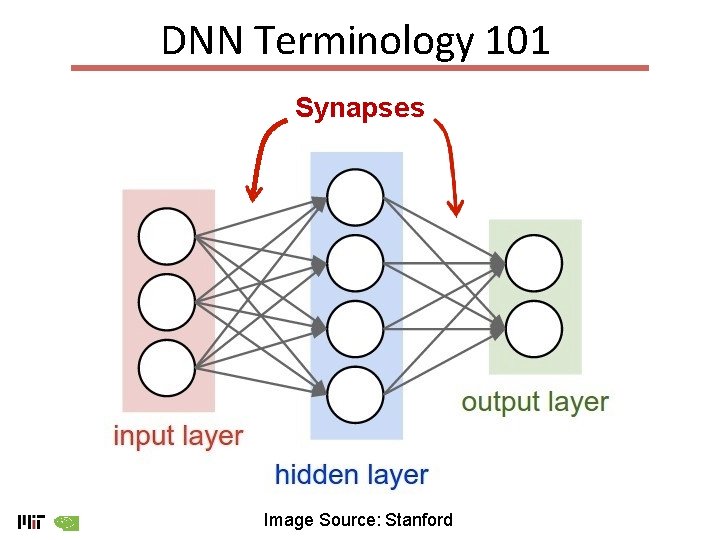
DNN Terminology 101 Synapses DNN Terminology 101 Image Source: Stanford

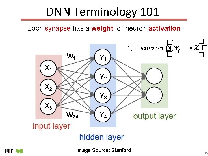
DNN Terminology 101 Each synapse has a weight for neuron activation W 11 Y 1 � 3 Y j activation � Wij � i 1 � Xi � � X 1 Y 2 X 2 Y 3 X 3 W 34 Y 4 Image Source: Stanford 45

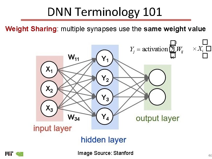
DNN Terminology 101 Weight Sharing: multiple synapses use the same weight value W 11 Y 1 � 3 Y j activation � Wij � i 1 � Xi � � X 1 Y 2 X 2 Y 3 X 3 W 34 Y 4 Image Source: Stanford 46

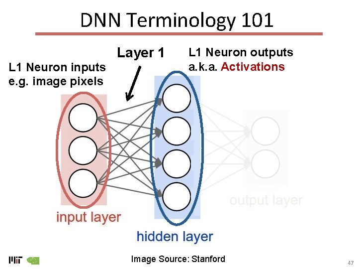
DNN Terminology 101 Layer 1 L 1 Neuron inputs e. g. image pixels L 1 Neuron outputs a. k. a. Activations Image Source: Stanford 47

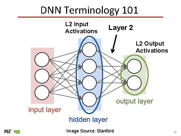
DNN Terminology 101 L 2 Input Activations Layer 2 L 2 Output Activations Image Source: Stanford 48

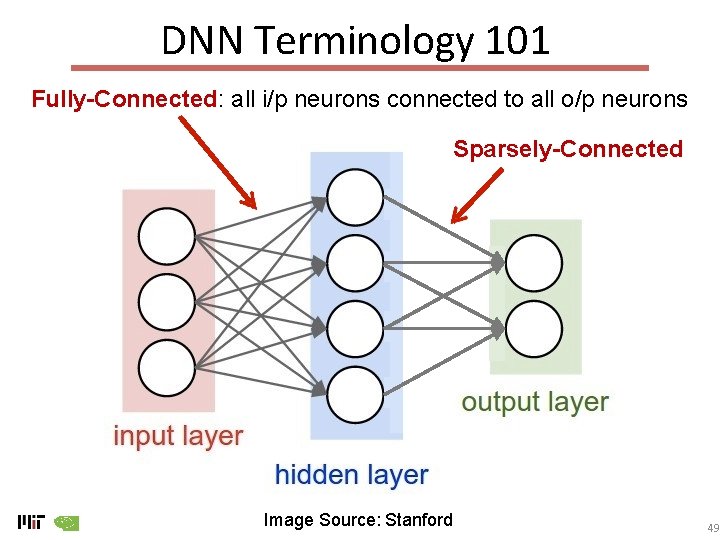
DNN Terminology 101 Fully-Connected: all i/p neurons connected to all o/p neurons Sparsely-Connected Image Source: Stanford 49

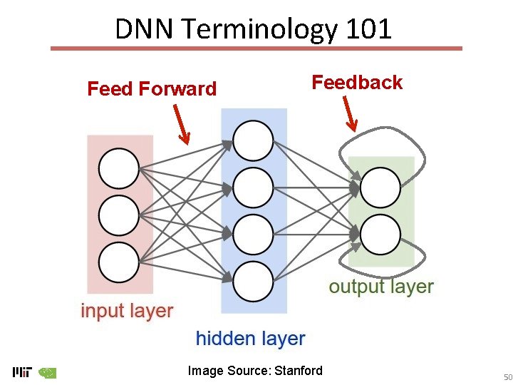
DNN Terminology 101 Feed Forward Feedback Image Source: Stanford 50

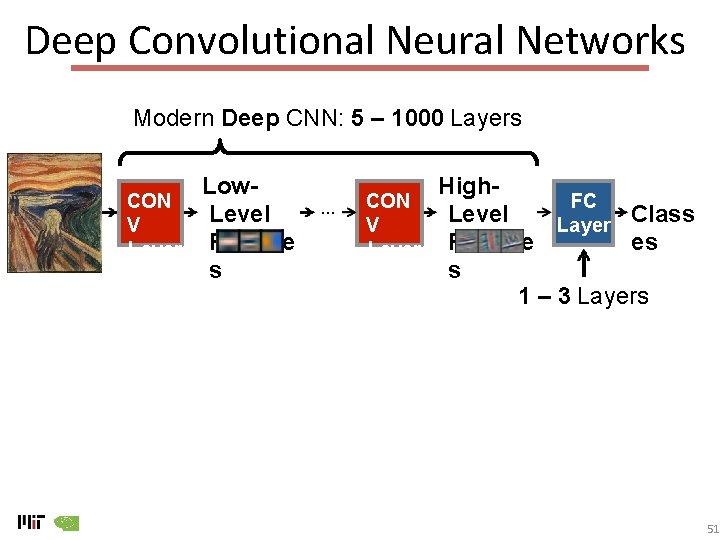
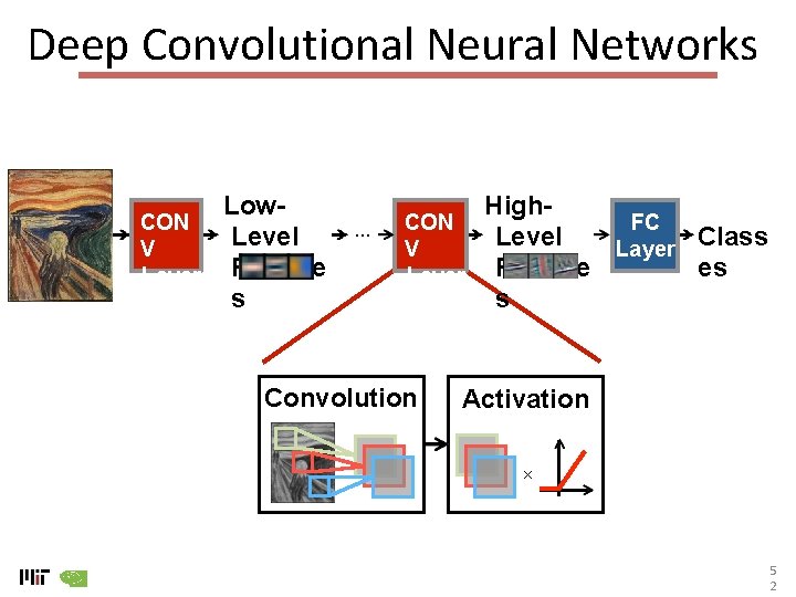
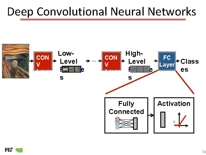
Deep Convolutional Neural Networks Modern Deep CNN: 5 – 1000 Layers Low. CON Level V Layer Feature s … High. CON FC Class Level V Layer es Layer Feature s 1 – 3 Layers 51

Deep Convolutional Neural Networks Low. CON Level V Layer Feature s … High. CON FC Class Level V Layer es Layer Feature s Convolution Activation × 5 2

Deep Convolutional Neural Networks Low. CON Level V Layer Feature s … High. CON FC Class Level V Layer es Layer Feature s Fully Connected Activation × 53

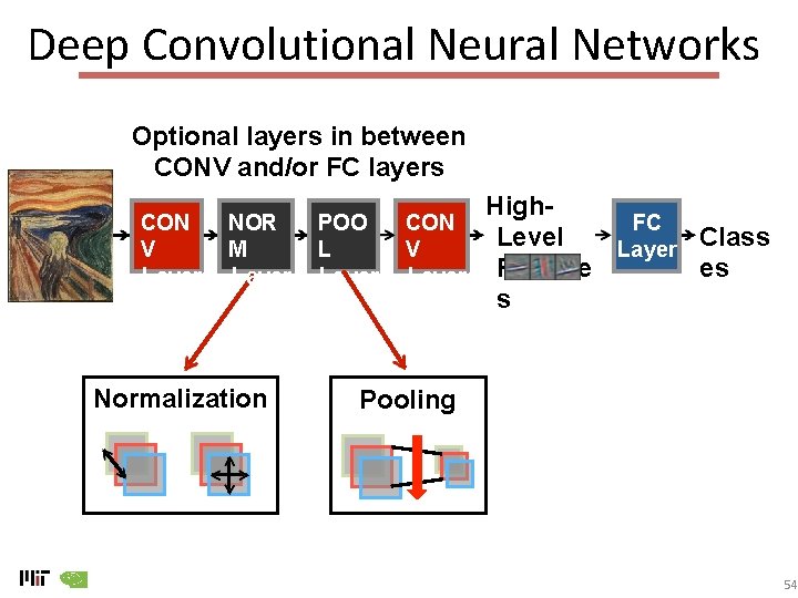
Deep Convolutional Neural Networks Optional layers in between CONV and/or FC layers CON V Layer NOR M Layer Normalization POO L Layer High. CON FC Class Level V Layer es Layer Feature s Pooling 54

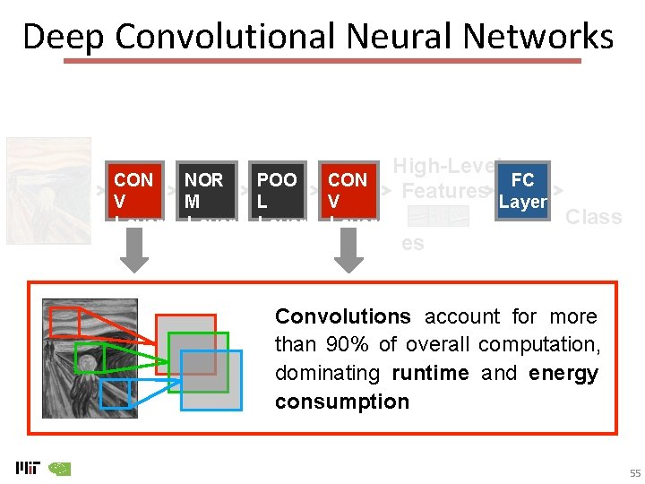
Deep Convolutional Neural Networks CON V Layer NOR M Layer POO L Layer CON V Layer High-Level FC Features Layer Class es Convolutions account for more than 90% of overall computation, dominating runtime and energy consumption 55

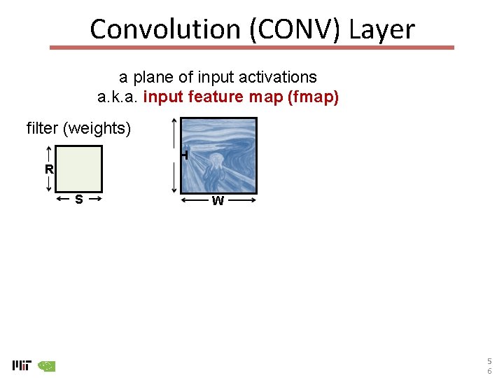
Convolution (CONV) Layer a plane of input activations a. k. a. input feature map (fmap) filter (weights) H R S W 5 6

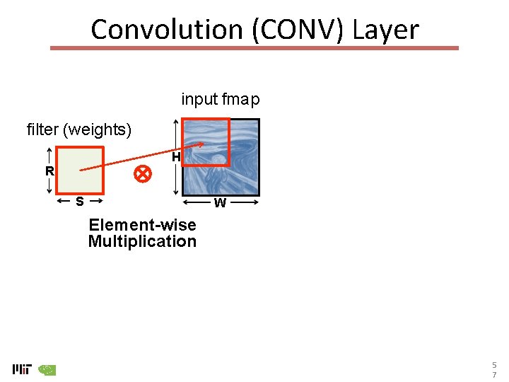
Convolution (CONV) Layer input fmap filter (weights) H R S W Element-wise Multiplication 5 7

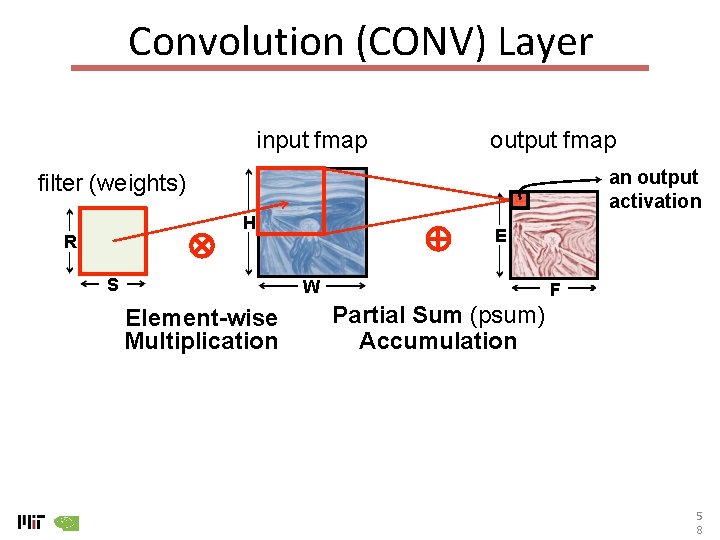
Convolution (CONV) Layer input fmap output fmap an output activation filter (weights) H R S E W Element-wise Multiplication F Partial Sum (psum) Accumulation 5 8

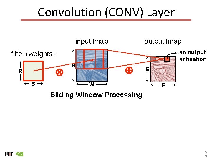
Convolution (CONV) Layer input fmap output fmap an output activation filter (weights) H R S E W F Sliding Window Processing 5 9

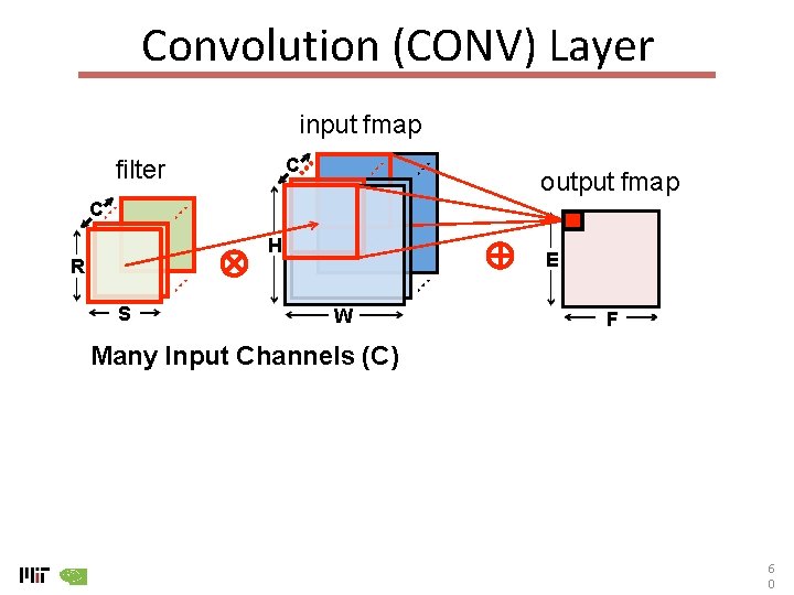
Convolution (CONV) Layer input fmap C filter output fmap C H R S E W F Many Input Channels (C) 6 0

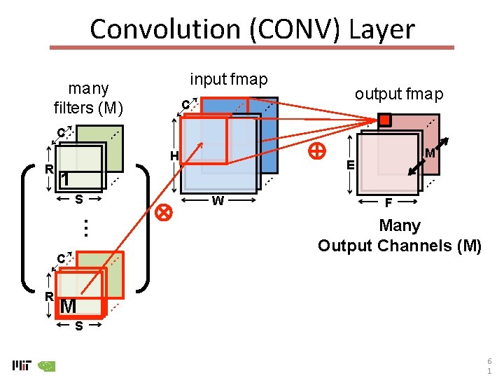
Convolution (CONV) Layer input fmap many filters (M) output fmap C C R H … C R E 1 S M W F Many Output Channels (M) M S 6 1

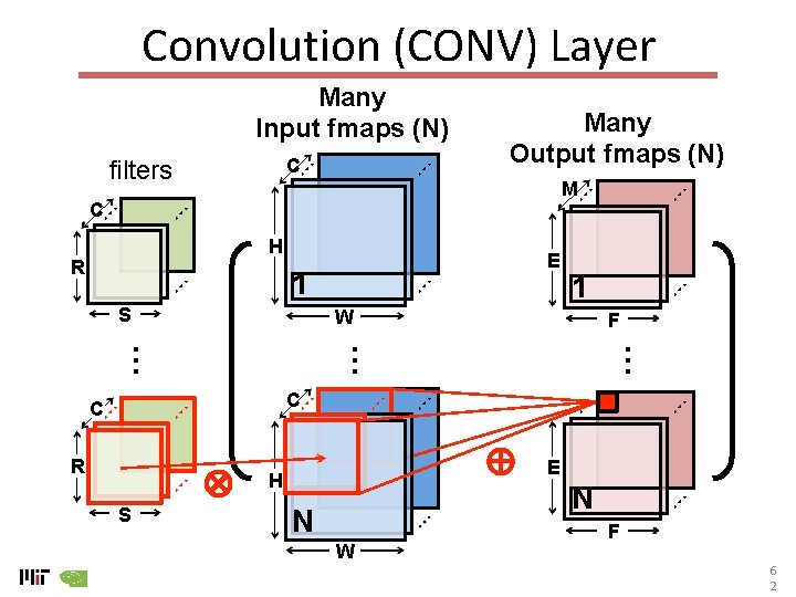
Convolution (CONV) Layer Many Input fmaps (N) C filters Many Output fmaps (N) M C H E 1 S 1 F … … W … R C C R E H S N N W F 6 2

How should we build an accelerator for the convolution layer? 63

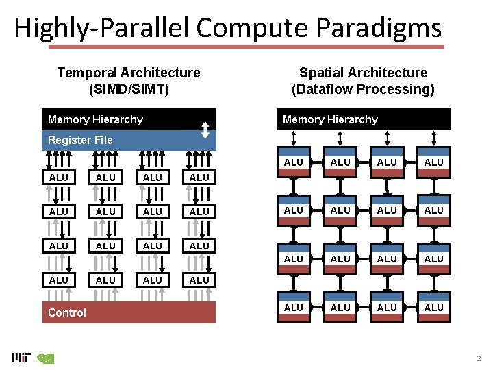
• What are the ways to take advantage of parallelism? – SIMD – Dataflow 64

Highly-Parallel Compute Paradigms Temporal Architecture (SIMD/SIMT) Memory Hierarchy Spatial Architecture (Dataflow Processing) Memory Hierarchy Register File ALU ALU ALU ALU Control ALU ALU ALU ALU ALU 2

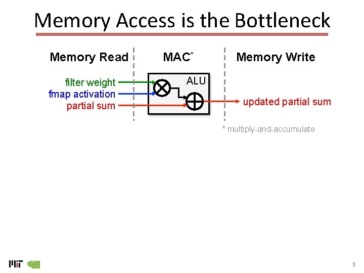
Memory Access is the Bottleneck Memory Read filter weight fmap activation partial sum MAC* Memory Write ALU updated partial sum * multiply-and-accumulate 3

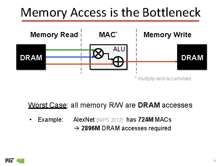
Memory Access is the Bottleneck Memory Read MAC* Memory Write ALU DRAM * multiply-and-accumulate Worst Case: all memory R/W are DRAM accesses • Example: Alex. Net [NIPS 2012] has 724 M MACs 2896 M DRAM accesses required 4

68

• What are the ways to address memory bottleneck? – Memory Hierarchy – Exploit locality 69

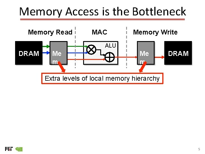
Memory Access is the Bottleneck Memory Read MAC Memory Write ALU DRAM Me m DRAM Extra levels of local memory hierarchy 5

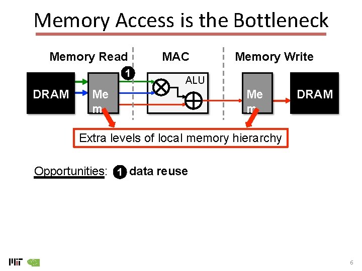
Memory Access is the Bottleneck Memory Read 1 DRAM MAC Memory Write ALU Me m DRAM Extra levels of local memory hierarchy Opportunities: 1 data reuse 6

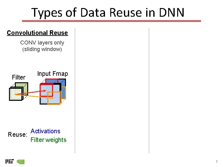
Types of Data Reuse in DNN Convolutional Reuse CONV layers only (sliding window) Filter Reuse: Input Fmap Activations Filter weights 7

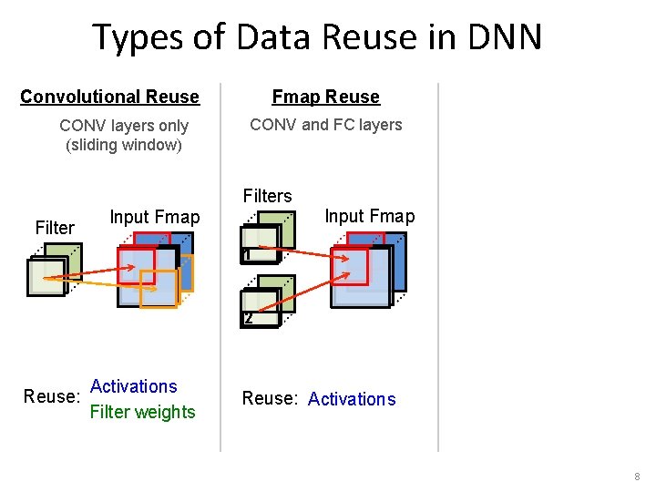
Types of Data Reuse in DNN Convolutional Reuse CONV layers only (sliding window) Fmap Reuse CONV and FC layers Filter Input Fmap 1 2 Reuse: Activations Filter weights Reuse: Activations 8

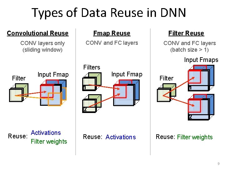
Types of Data Reuse in DNN Convolutional Reuse CONV layers only (sliding window) Fmap Reuse CONV and FC layers Filter Reuse CONV and FC layers (batch size > 1) Input Fmaps Filter Input Fmap 1 Filter 1 2 2 Reuse: Activations Filter weights Reuse: Activations Reuse: Filter weights 9

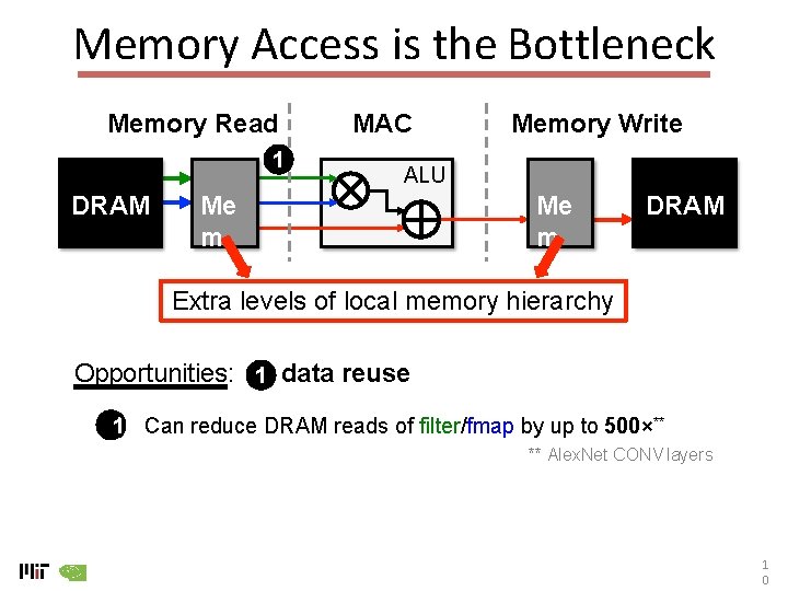
Memory Access is the Bottleneck Memory Read 1 DRAM MAC Memory Write ALU Me m DRAM Extra levels of local memory hierarchy Opportunities: 1 data reuse 11) Can reduce DRAM reads of filter/fmap by up to 500×** ** Alex. Net CONV layers 1 0

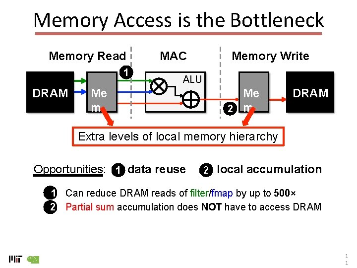
Memory Access is the Bottleneck Memory Read 1 DRAM MAC Memory Write ALU Me m Me 2 m DRAM Extra levels of local memory hierarchy Opportunities: 1 data reuse 2 local accumulation 11) Can reduce DRAM reads of filter/fmap by up to 500× 22) Partial sum accumulation does NOT have to access DRAM 1 1

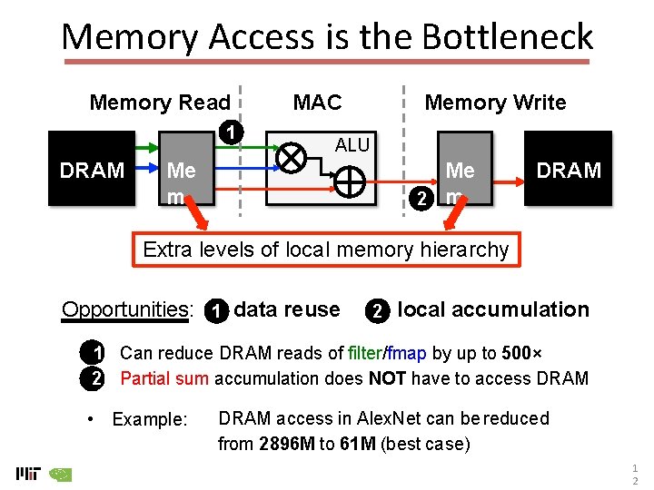
Memory Access is the Bottleneck Memory Read 1 DRAM MAC Memory Write ALU Me m Me 2 m DRAM Extra levels of local memory hierarchy Opportunities: 1 data reuse 2 local accumulation 11) Can reduce DRAM reads of filter/fmap by up to 500× 22) Partial sum accumulation does NOT have to access DRAM • Example: DRAM access in Alex. Net can be reduced from 2896 M to 61 M (best case) 1 2

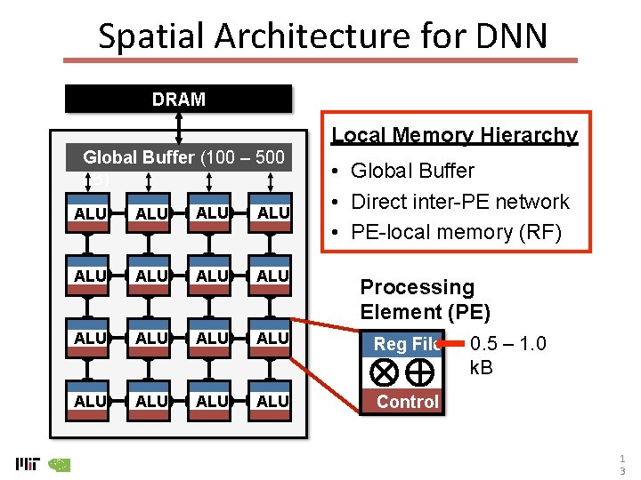
Spatial Architecture for DNN DRAM Local Memory Hierarchy Global Buffer (100 – 500 k. B) • Global Buffer • Direct inter-PE network • PE-local memory (RF) ALU ALU ALU Reg File ALU ALU Control Processing Element (PE) 0. 5 – 1. 0 k. B 1 3

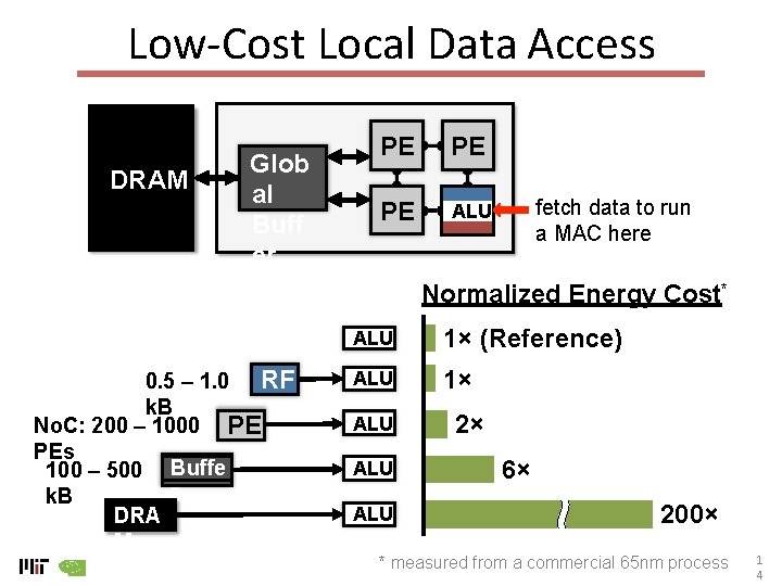
Low-Cost Local Data Access DRAM Glob al Buff er PE PE PE ALU fetch data to run a MAC here Normalized Energy Cost* 0. 5 – 1. 0 RF k. B No. C: 200 – 1000 PE PEs 100 – 500 Buffe r k. B DRA M ALU 1× (Reference) ALU 1× ALU ALU 2× 6× 200× * measured from a commercial 65 nm process 1 4

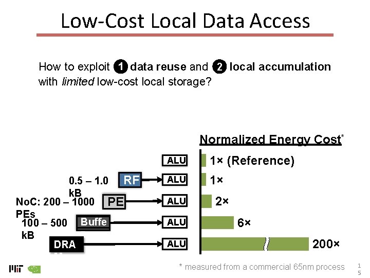
Low-Cost Local Data Access How to exploit 1 data reuse and 2 local accumulation with limited low-cost local storage? Normalized Energy Cost* 0. 5 – 1. 0 RF k. B No. C: 200 – 1000 PE PEs 100 – 500 Buffe r k. B DRA M ALU 1× (Reference) ALU 1× ALU ALU 2× 6× 200× * measured from a commercial 65 nm process 1 5

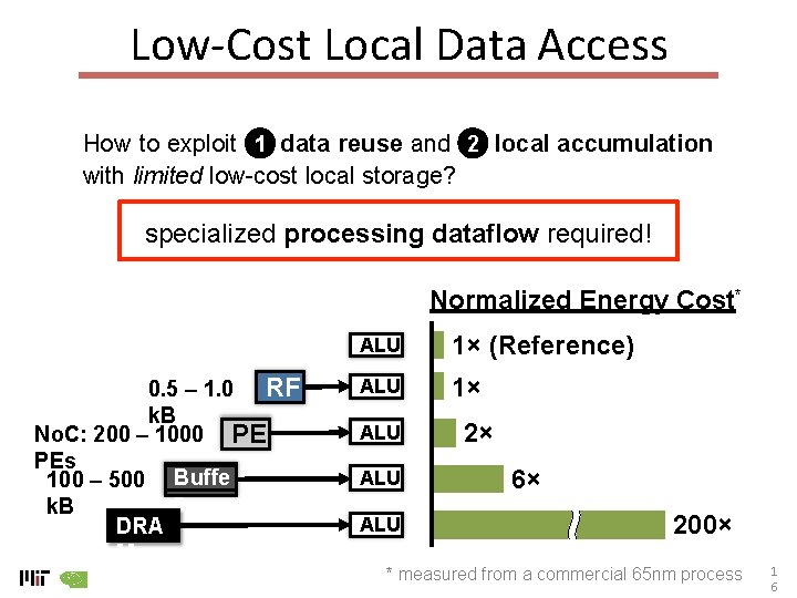
Low-Cost Local Data Access How to exploit 1 data reuse and 2 local accumulation with limited low-cost local storage? specialized processing dataflow required! Normalized Energy Cost* 0. 5 – 1. 0 RF k. B No. C: 200 – 1000 PE PEs 100 – 500 Buffe r k. B DRA M ALU 1× (Reference) ALU 1× ALU ALU 2× 6× 200× * measured from a commercial 65 nm process 1 6

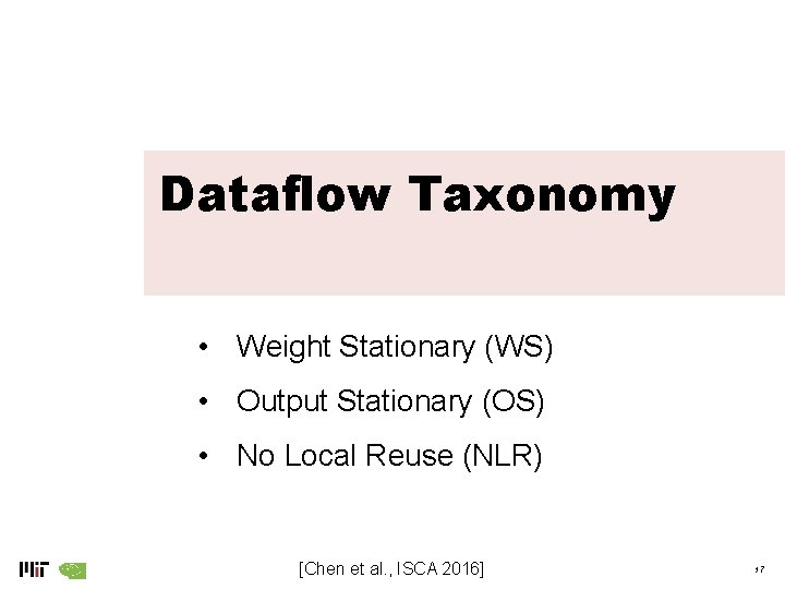
Dataflow Taxonomy • Weight Stationary (WS) • Output Stationary (OS) • No Local Reuse (NLR) [Chen et al. , ISCA 2016] 17

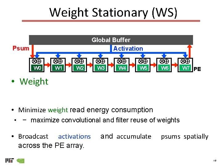
Weight Stationary (WS) Global Buffer Activation Psum W 0 W 1 W 2 W 3 W 4 W 5 W 6 W 7 PE • Weight • Minimize weight read energy consumption • − maximize convolutional and filter reuse of weights • Broadcast activations across the PE array. and accumulate psums spatially 18

ADVANCED COMPUTER ARCHITECTURE ML Accelerators: Why Samira Khan University of Virginia Feb 4, 2019 The content and concept of this course are adapted from CMU ECE 740