CSE 160 Lecture 9 Speedup Amdahls Law Gustafsons

CSE 160 – Lecture 9 Speed-up, Amdahl’s Law, Gustafson’s Law, efficiency, basic performance metrics

Exam 1 • 9 May 2000, 1 week from today • Covers material through HW#2 + through Amdahl’s law/Efficiency in this lecture • Closed book, Closed Notes. You may use a calculator. • At the end of this lecture –will ask you for a list of things you want reviewed during next lecture.

Concurrency/Granularity • One key to efficient parallel programming is concurrency. • For parallel tasks we talk about the granularity – size of the computation between synchronization points – Coarse – heavyweight processes + IPC (interprocess communication (PVM, MPI, … ) – Fine – Instruction level (eg. SIMD) – Medium – Threads + [message passing + shared memory synch]

One measurement of granularity • Computation to Communication Ratio – (Computation time)/(Communication time) – Increasing this ratio is often a key to good efficiency – How does this measure granularity? • CCR = ? Grain

Communication Overhead • Another important metric is communication overhead – time (measured in instructions) a zerobyte message consumes in a process – Measure time spent on communication that cannot be spent on computation • Overlapped Messages – portion of message lifetime that can occur concurrently with computation – time bits are on wire – time bits are in the switch or NIC

Many little things add up … • Lots of little things add up that add overhead to a parallel program – Efficient implementations demand • Overlapping (aka hiding) the overheads as much as possible • Keeping non-overlapping overheads as small as possible

Speed-Up • S(n) = – (Execution time on Single CPU)/(Execution on N parallel processors) – ts /tp – Serial time is for best serial algorithm • This may be a different algorithm than a parallel version – Divide-and-conquer Quicksort O(Nlog. N) vs. Mergesort

Linear and Superlinear Speedup • Linear speedup = N, for N processors – Parallel program is perfectly scalable – Rarely achieved in practice • Superlinear Speedup – S(N) > N for N processors • Theoretically not possible • How is this achievable on real machines? – Think about physical resources of N processors

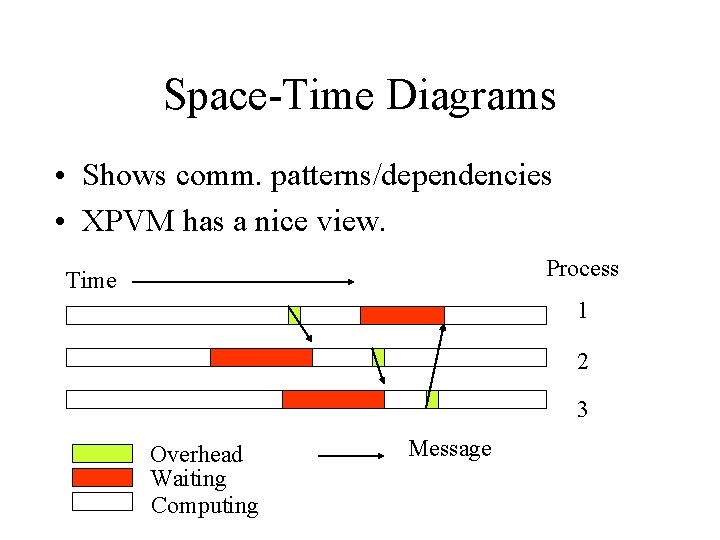
Space-Time Diagrams • Shows comm. patterns/dependencies • XPVM has a nice view. Process Time 1 2 3 Overhead Waiting Computing Message

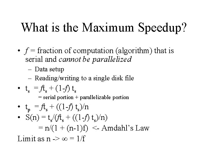
What is the Maximum Speedup? • f = fraction of computation (algorithm) that is serial and cannot be parallelized – Data setup – Reading/writing to a single disk file • ts = fts + (1 -f) ts = serial portion + parallelizable portion • tp = fts + ((1 -f) ts)/n • S(n) = ts/(fts + ((1 -f) ts)/n) = n/(1 + (n-1)f) <- Amdahl’s Law Limit as n -> = 1/f

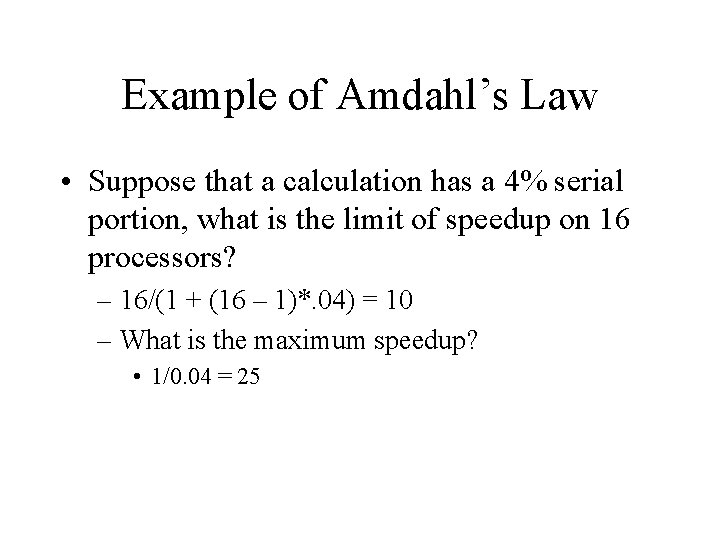
Example of Amdahl’s Law • Suppose that a calculation has a 4% serial portion, what is the limit of speedup on 16 processors? – 16/(1 + (16 – 1)*. 04) = 10 – What is the maximum speedup? • 1/0. 04 = 25

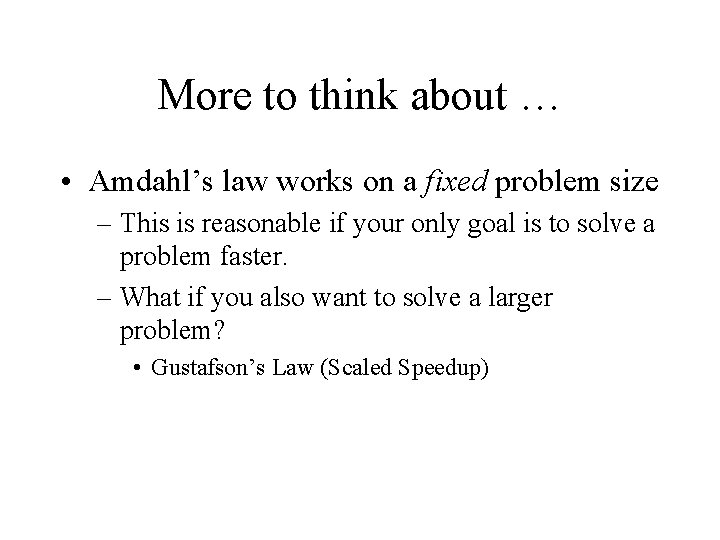
More to think about … • Amdahl’s law works on a fixed problem size – This is reasonable if your only goal is to solve a problem faster. – What if you also want to solve a larger problem? • Gustafson’s Law (Scaled Speedup)

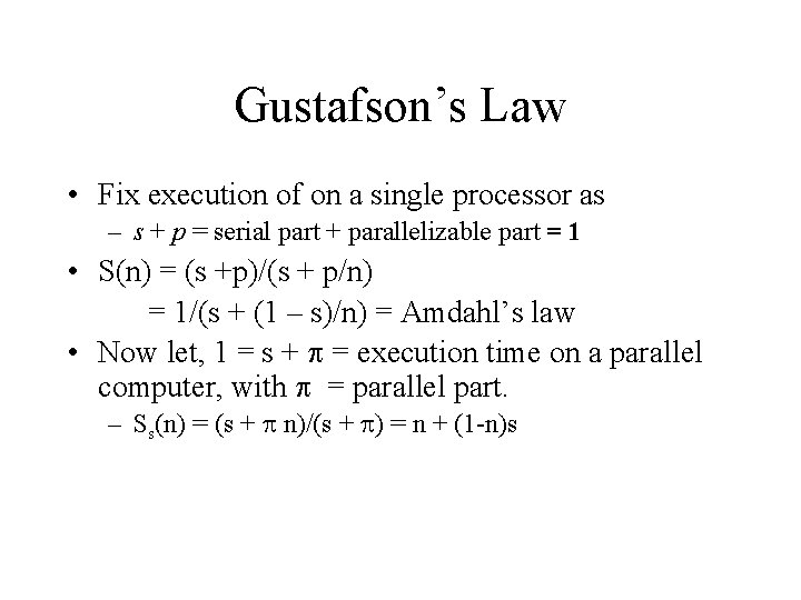
Gustafson’s Law • Fix execution of on a single processor as – s + p = serial part + parallelizable part = 1 • S(n) = (s +p)/(s + p/n) = 1/(s + (1 – s)/n) = Amdahl’s law • Now let, 1 = s + = execution time on a parallel computer, with = parallel part. – Ss(n) = (s + n)/(s + ) = n + (1 -n)s

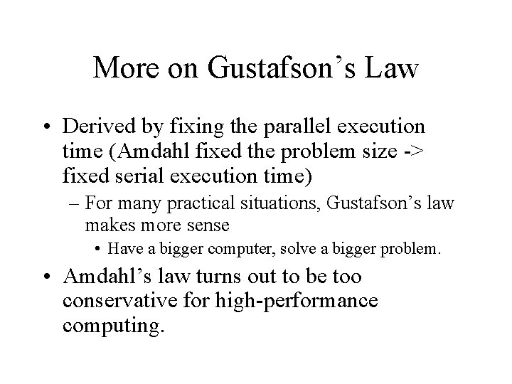
More on Gustafson’s Law • Derived by fixing the parallel execution time (Amdahl fixed the problem size -> fixed serial execution time) – For many practical situations, Gustafson’s law makes more sense • Have a bigger computer, solve a bigger problem. • Amdahl’s law turns out to be too conservative for high-performance computing.

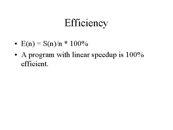
Efficiency • E(n) = S(n)/n * 100% • A program with linear speedup is 100% efficient.

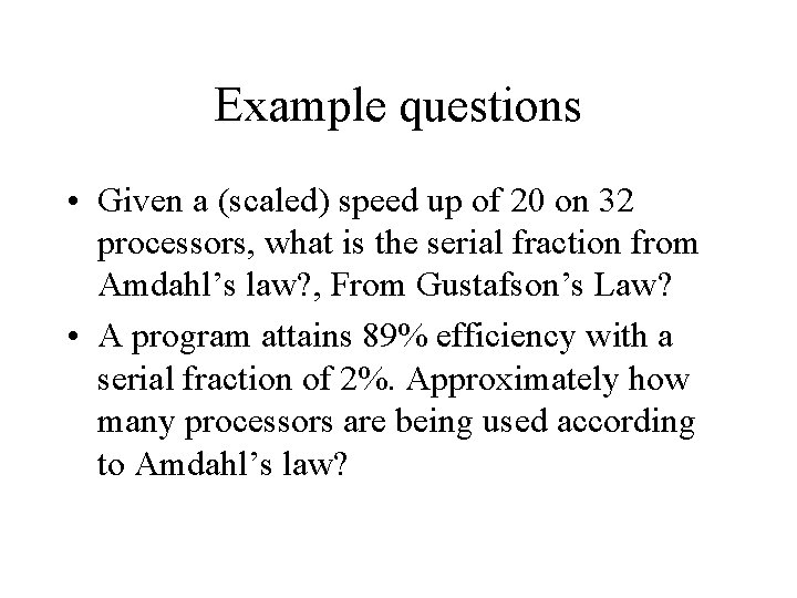
Example questions • Given a (scaled) speed up of 20 on 32 processors, what is the serial fraction from Amdahl’s law? , From Gustafson’s Law? • A program attains 89% efficiency with a serial fraction of 2%. Approximately how many processors are being used according to Amdahl’s law?

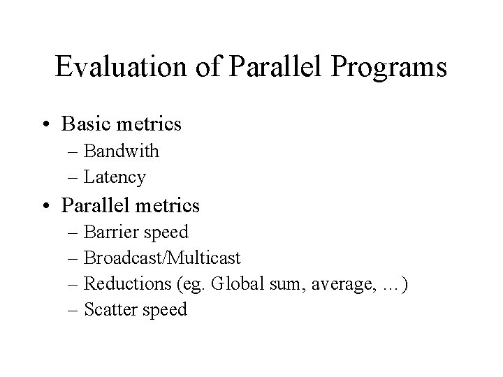
Evaluation of Parallel Programs • Basic metrics – Bandwith – Latency • Parallel metrics – Barrier speed – Broadcast/Multicast – Reductions (eg. Global sum, average, …) – Scatter speed

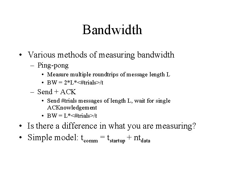
Bandwidth • Various methods of measuring bandwidth – Ping-pong • Measure multiple roundtrips of message length L • BW = 2*L*<#trials>/t – Send + ACK • Send #trials messages of length L, wait for single ACKnowledgement • BW = L*<#trials>/t • Is there a difference in what you are measuring? • Simple model: tcomm = tstartup + ntdata

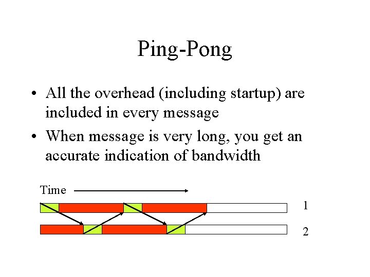
Ping-Pong • All the overhead (including startup) are included in every message • When message is very long, you get an accurate indication of bandwidth Time 1 2

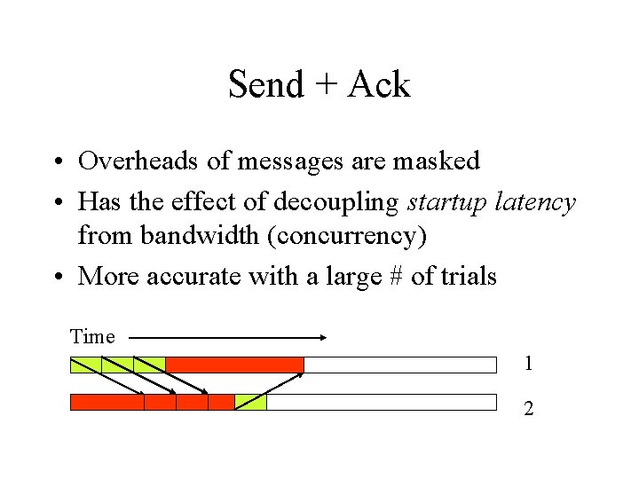
Send + Ack • Overheads of messages are masked • Has the effect of decoupling startup latency from bandwidth (concurrency) • More accurate with a large # of trials Time 1 2

In the limit … • As messages get larger, both methods converge to the same number • How does one measure latency? – Ping-pong over multiple trials – Latency = 2*<#ntrials>/t • What things aren’t being measured (or are being smeared by these two methods)? – Will talk about cost models and the start of Log. P analysis next time.

How you measure performance • It is important to understand exactly what you are measuring and how you are measuring it.

Exam … • What topics/questions do you want reviewed? • Are there specific questions on the homework/programming assignment that need talking about?

Questions • Go over programming assignment #1 • Go over programming assignment #2