Advanced Compilers CMPSCI 710 Spring 2003 Computing SSA

Advanced Compilers CMPSCI 710 Spring 2003 Computing SSA Emery Berger University of Massachusetts, Amherst UNIVERSITY OF MASSACHUSETTS, AMHERST • DEPARTMENT OF COMPUTER SCIENCE

More SSA n Last time n n n dominance SSA form Today n Computing SSA form UNIVERSITY OF MASSACHUSETTS, AMHERST • DEPARTMENT OF COMPUTER SCIENCE 2

Criteria for Inserting Functions n Brute-force: Insert one function for each variable at every join point (point in CFG with more than one predecessor) n n Wasteful When should we insert function for a variable a at node z of the CFG? n Intuitively: add if there are two definitions of a that can reach the point z through distinct paths UNIVERSITY OF MASSACHUSETTS, AMHERST • DEPARTMENT OF COMPUTER SCIENCE 3

Path Convergence Criterion [Cytron-Ferrante ‘ 89] Insert function for variable a at node z if all the following conditions are true: 1. There is a block x that defines a 2. There is a block y x that defines a 3. There are non-empty paths x z and y z 4. Paths x z and y z don’t have nodes in common other than z 5. The node z does not appear within both x z and y z prior to the end, but it may appear in one or the other. Note: The start node contains an implicit definition of every variable. UNIVERSITY OF MASSACHUSETTS, AMHERST • DEPARTMENT OF COMPUTER SCIENCE 4

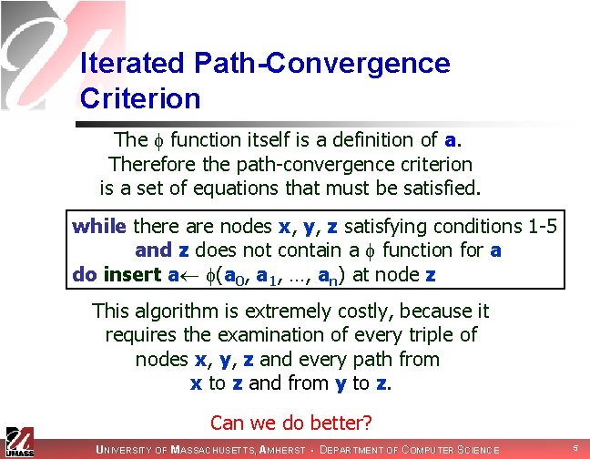
Iterated Path-Convergence Criterion The function itself is a definition of a. Therefore the path-convergence criterion is a set of equations that must be satisfied. while there are nodes x, y, z satisfying conditions 1 -5 and z does not contain a function for a do insert a (a 0, a 1, …, an) at node z This algorithm is extremely costly, because it requires the examination of every triple of nodes x, y, z and every path from x to z and from y to z. Can we do better? UNIVERSITY OF MASSACHUSETTS, AMHERST • DEPARTMENT OF COMPUTER SCIENCE 5

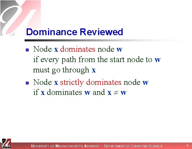
Dominance Reviewed n n Node x dominates node w if every path from the start node to w must go through x Node x strictly dominates node w if x dominates w and x w UNIVERSITY OF MASSACHUSETTS, AMHERST • DEPARTMENT OF COMPUTER SCIENCE 6

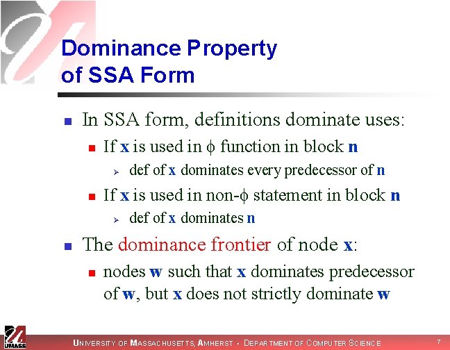
Dominance Property of SSA Form n In SSA form, definitions dominate uses: n If x is used in function in block n Ø n If x is used in non- statement in block n Ø n def of x dominates every predecessor of n def of x dominates n The dominance frontier of node x: n nodes w such that x dominates predecessor of w, but x does not strictly dominate w UNIVERSITY OF MASSACHUSETTS, AMHERST • DEPARTMENT OF COMPUTER SCIENCE 7

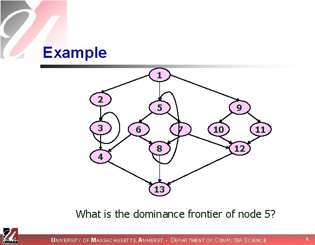
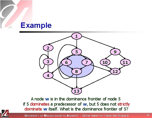
Example 1 2 3 4 5 6 9 7 8 10 11 12 13 What is the dominance frontier of node 5? UNIVERSITY OF MASSACHUSETTS, AMHERST • DEPARTMENT OF COMPUTER SCIENCE 8

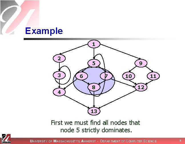
Example 1 2 3 4 5 6 9 7 8 10 11 12 13 First we must find all nodes that node 5 strictly dominates. UNIVERSITY OF MASSACHUSETTS, AMHERST • DEPARTMENT OF COMPUTER SCIENCE 9

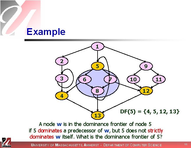
Example 1 2 3 4 5 6 9 7 8 10 11 12 13 A node w is in the dominance frontier of node 5 if 5 dominates a predecessor of w, but 5 does not strictly dominate w itself. What is the dominance frontier of 5? UNIVERSITY OF MASSACHUSETTS, AMHERST • DEPARTMENT OF COMPUTER SCIENCE 10

Example 1 2 3 4 5 6 9 7 8 13 10 11 12 DF(5) = {4, 5, 12, 13} A node w is in the dominance frontier of node 5 if 5 dominates a predecessor of w, but 5 does not strictly dominates w itself. What is the dominance frontier of 5? UNIVERSITY OF MASSACHUSETTS, AMHERST • DEPARTMENT OF COMPUTER SCIENCE 11

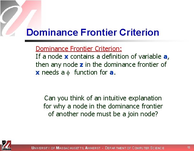
Dominance Frontier Criterion: If a node x contains a definition of variable a, then any node z in the dominance frontier of x needs a function for a. Can you think of an intuitive explanation for why a node in the dominance frontier of another node must be a join node? UNIVERSITY OF MASSACHUSETTS, AMHERST • DEPARTMENT OF COMPUTER SCIENCE 12

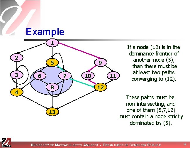
Example 1 2 3 4 5 6 9 7 8 13 10 11 If a node (12) is in the dominance frontier of another node (5), than there must be at least two paths converging to (12). 12 These paths must be non-intersecting, and one of them (5, 7, 12) must contain a node strictly dominated by (5). UNIVERSITY OF MASSACHUSETTS, AMHERST • DEPARTMENT OF COMPUTER SCIENCE 13

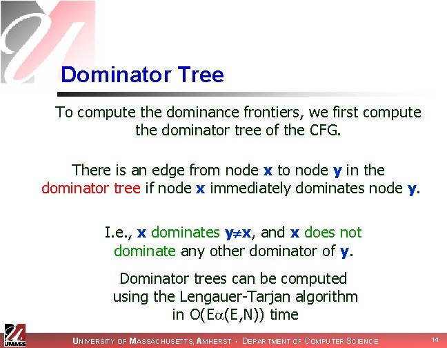
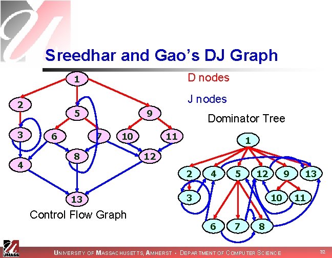
Dominator Tree To compute the dominance frontiers, we first compute the dominator tree of the CFG. There is an edge from node x to node y in the dominator tree if node x immediately dominates node y. I. e. , x dominates y x, and x does not dominate any other dominator of y. Dominator trees can be computed using the Lengauer-Tarjan algorithm in O(E (E, N)) time UNIVERSITY OF MASSACHUSETTS, AMHERST • DEPARTMENT OF COMPUTER SCIENCE 14

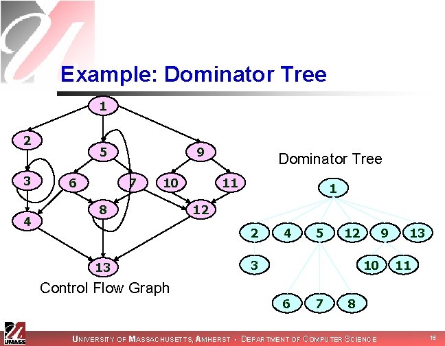
Example: Dominator Tree 1 2 3 4 5 6 9 7 10 8 Dominator Tree 11 1 12 2 13 Control Flow Graph 4 5 12 3 9 10 6 7 13 11 8 UNIVERSITY OF MASSACHUSETTS, AMHERST • DEPARTMENT OF COMPUTER SCIENCE 15

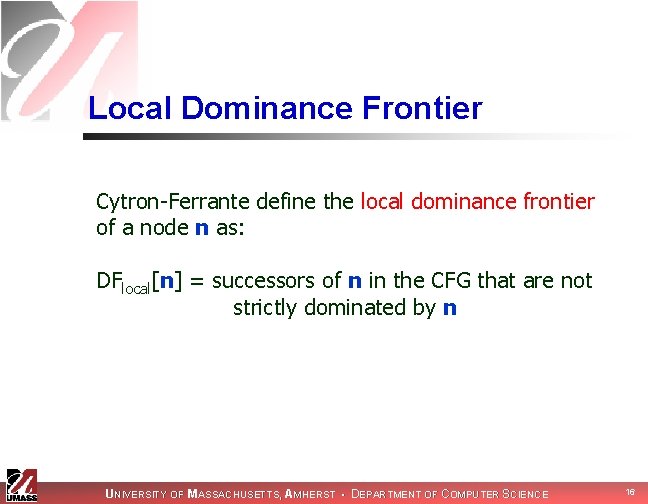
Local Dominance Frontier Cytron-Ferrante define the local dominance frontier of a node n as: DFlocal[n] = successors of n in the CFG that are not strictly dominated by n UNIVERSITY OF MASSACHUSETTS, AMHERST • DEPARTMENT OF COMPUTER SCIENCE 16

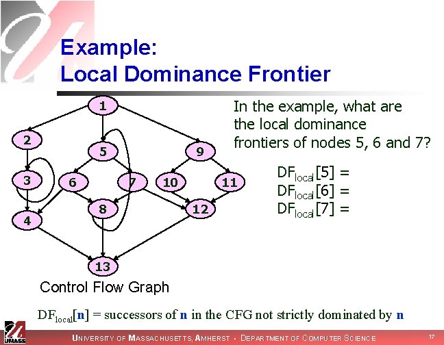
Example: Local Dominance Frontier 1 2 3 4 5 6 9 7 10 8 In the example, what are the local dominance frontiers of nodes 5, 6 and 7? 11 12 DFlocal[5] = DFlocal[6] = {4, 8} DFlocal[7] = {8, 12} 13 Control Flow Graph DFlocal[n] = successors of n in the CFG not strictly dominated by n UNIVERSITY OF MASSACHUSETTS, AMHERST • DEPARTMENT OF COMPUTER SCIENCE 17

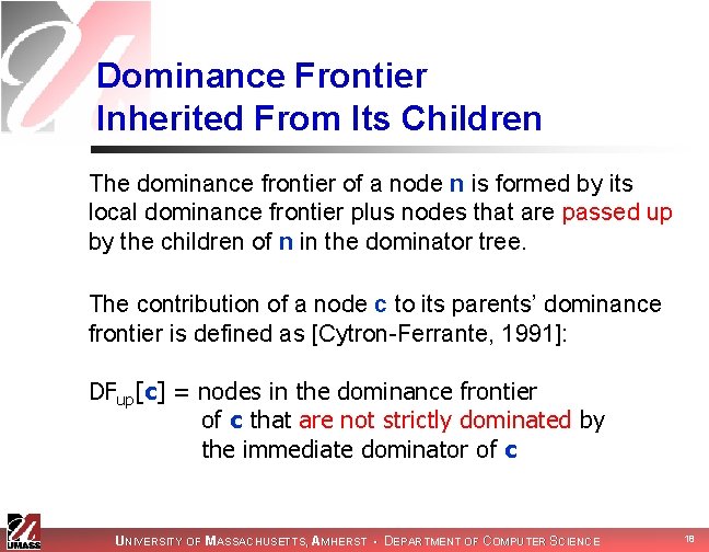
Dominance Frontier Inherited From Its Children The dominance frontier of a node n is formed by its local dominance frontier plus nodes that are passed up by the children of n in the dominator tree. The contribution of a node c to its parents’ dominance frontier is defined as [Cytron-Ferrante, 1991]: DFup[c] = nodes in the dominance frontier of c that are not strictly dominated by the immediate dominator of c UNIVERSITY OF MASSACHUSETTS, AMHERST • DEPARTMENT OF COMPUTER SCIENCE 18

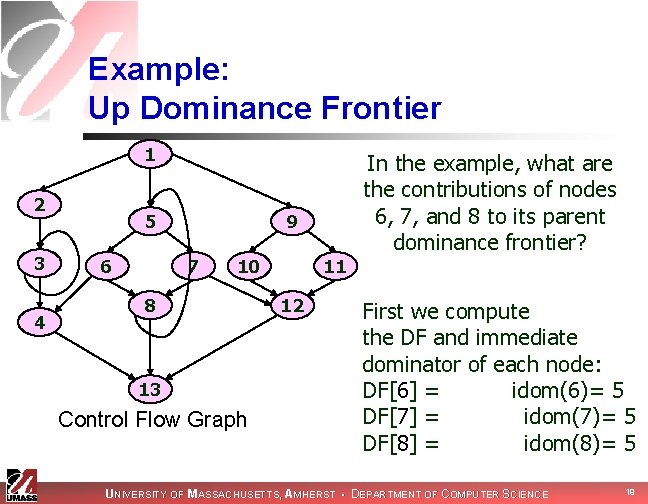
Example: Up Dominance Frontier 1 2 3 4 5 6 In the example, what are the contributions of nodes 6, 7, and 8 to its parent dominance frontier? 9 7 10 8 13 Control Flow Graph 11 12 First we compute the DF and immediate dominator of each node: DF[6] = {4, 8}, idom(6)= 5 DF[7] = {8, 12}, idom(7)= 5 DF[8] = {5, 13}, idom(8)= 5 UNIVERSITY OF MASSACHUSETTS, AMHERST • DEPARTMENT OF COMPUTER SCIENCE 19

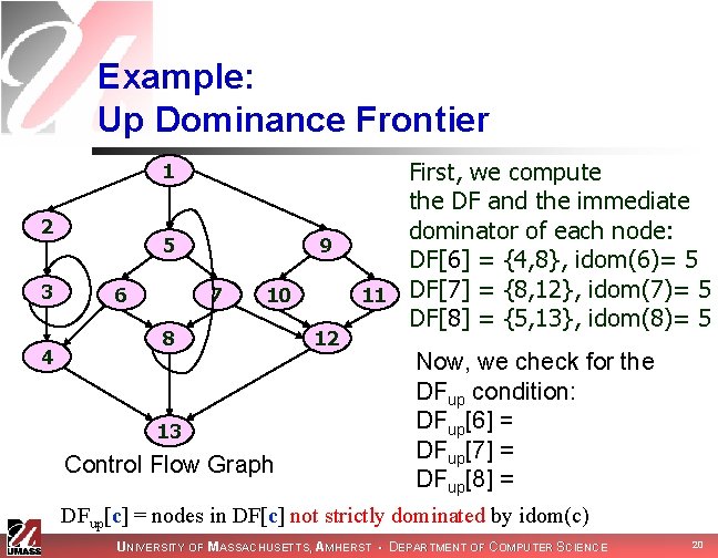
Example: Up Dominance Frontier 1 2 3 4 5 6 9 7 10 8 13 Control Flow Graph 12 First, we compute the DF and the immediate dominator of each node: DF[6] = {4, 8}, idom(6)= 5 11 DF[7] = {8, 12}, idom(7)= 5 DF[8] = {5, 13}, idom(8)= 5 Now, we check for the DFup condition: DFup[6] = {4} DFup[7] = {12} DFup[8] = {5, 13} DFup[c] = nodes in DF[c] not strictly dominated by idom(c) UNIVERSITY OF MASSACHUSETTS, AMHERST • DEPARTMENT OF COMPUTER SCIENCE 20

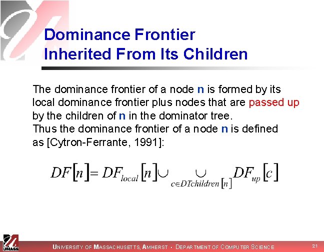
Dominance Frontier Inherited From Its Children The dominance frontier of a node n is formed by its local dominance frontier plus nodes that are passed up by the children of n in the dominator tree. Thus the dominance frontier of a node n is defined as [Cytron-Ferrante, 1991]: UNIVERSITY OF MASSACHUSETTS, AMHERST • DEPARTMENT OF COMPUTER SCIENCE 21

Example: Local Dominance Frontier 1 2 3 4 What is DF[5]? 5 6 Remember that: 9 7 10 8 11 12 DFlocal[5] = DFup[6] = {4} DFup[7] = {12} DFup[8] = {5, 13} DTchildren[5] = {6, 7, 8} 13 Control Flow Graph UNIVERSITY OF MASSACHUSETTS, AMHERST • DEPARTMENT OF COMPUTER SCIENCE 22

Example: Local Dominance Frontier 1 2 3 4 What is DF[5]? 5 6 Remember that: 9 7 10 8 11 12 DFlocal[5] = DFup[6] = {4} DFup[7] = {12} DFup[8] = {5, 13} DTchildren[5] = {6, 7, 8} 13 Control Flow Graph Thus, DF[5] = {4, 5, 12, 13} UNIVERSITY OF MASSACHUSETTS, AMHERST • DEPARTMENT OF COMPUTER SCIENCE 23

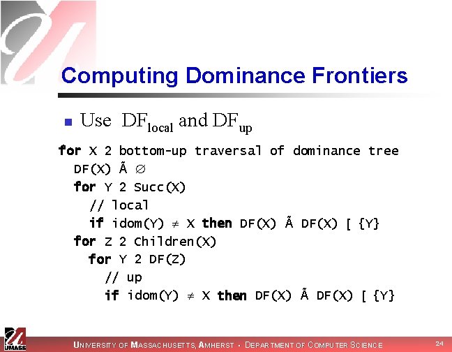
Computing Dominance Frontiers n Use DFlocal and DFup for X 2 bottom-up traversal of dominance tree DF(X) Ã for Y 2 Succ(X) // local if idom(Y) X then DF(X) Ã DF(X) [ {Y} for Z 2 Children(X) for Y 2 DF(Z) // up if idom(Y) X then DF(X) Ã DF(X) [ {Y} UNIVERSITY OF MASSACHUSETTS, AMHERST • DEPARTMENT OF COMPUTER SCIENCE 24

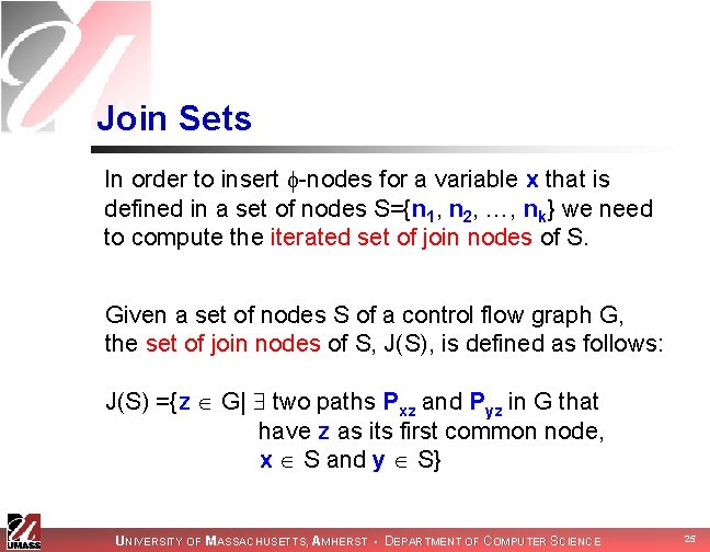
Join Sets In order to insert -nodes for a variable x that is defined in a set of nodes S={n 1, n 2, …, nk} we need to compute the iterated set of join nodes of S. Given a set of nodes S of a control flow graph G, the set of join nodes of S, J(S), is defined as follows: J(S) ={z G| two paths Pxz and Pyz in G that have z as its first common node, x S and y S} UNIVERSITY OF MASSACHUSETTS, AMHERST • DEPARTMENT OF COMPUTER SCIENCE 25

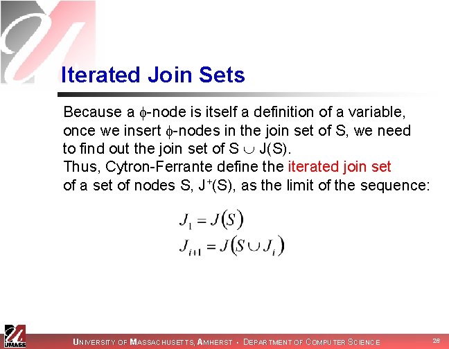
Iterated Join Sets Because a -node is itself a definition of a variable, once we insert -nodes in the join set of S, we need to find out the join set of S J(S). Thus, Cytron-Ferrante define the iterated join set of a set of nodes S, J+(S), as the limit of the sequence: UNIVERSITY OF MASSACHUSETTS, AMHERST • DEPARTMENT OF COMPUTER SCIENCE 26

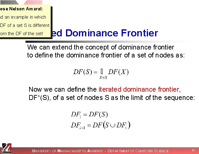
Jose Nelson Amaral: nd an example in which IDF of a set S is different Iterated Dominance Frontier rom the DF of the set! We can extend the concept of dominance frontier to define the dominance frontier of a set of nodes as: Now we can define the iterated dominance frontier, DF+(S), of a set of nodes S as the limit of the sequence: UNIVERSITY OF MASSACHUSETTS, AMHERST • DEPARTMENT OF COMPUTER SCIENCE 27

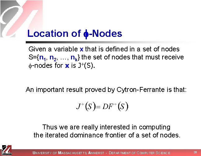
Location of -Nodes Given a variable x that is defined in a set of nodes S={n 1, n 2, …, nk} the set of nodes that must receive -nodes for x is J+(S). An important result proved by Cytron-Ferrante is that: Thus we are really interested in computing the iterated dominance frontier of a set of nodes. UNIVERSITY OF MASSACHUSETTS, AMHERST • DEPARTMENT OF COMPUTER SCIENCE 28

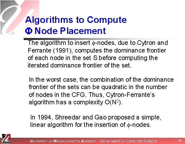
Algorithms to Compute Node Placement The algorithm to insert -nodes, due to Cytron and Ferrante (1991), computes the dominance frontier of each node in the set S before computing the iterated dominance frontier of the set. In the worst case, the combination of the dominance frontier of the sets can be quadratic in the number of nodes in the CFG. Thus, Cytron-Ferrante’s algorithm has a complexity O(N 2). In 1994, Shreedar and Gao proposed a simple, linear algorithm for the insertion of -nodes. UNIVERSITY OF MASSACHUSETTS, AMHERST • DEPARTMENT OF COMPUTER SCIENCE 29

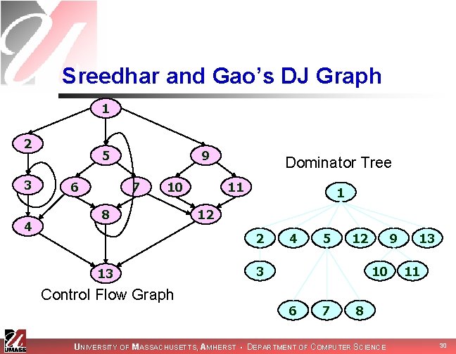
Sreedhar and Gao’s DJ Graph 1 2 3 4 5 6 9 7 10 8 Dominator Tree 11 1 12 2 13 Control Flow Graph 4 5 12 3 9 10 6 7 13 11 8 UNIVERSITY OF MASSACHUSETTS, AMHERST • DEPARTMENT OF COMPUTER SCIENCE 30

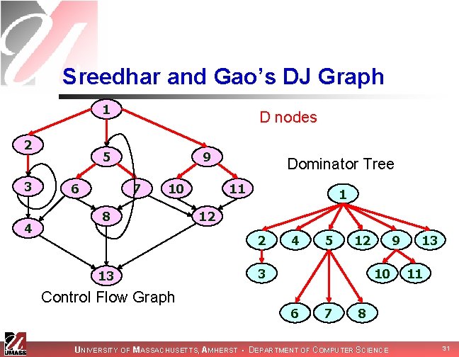
Sreedhar and Gao’s DJ Graph 1 2 3 4 D nodes 5 6 9 7 10 8 Dominator Tree 11 1 12 2 13 Control Flow Graph 4 5 12 3 9 10 6 7 13 11 8 UNIVERSITY OF MASSACHUSETTS, AMHERST • DEPARTMENT OF COMPUTER SCIENCE 31

Sreedhar and Gao’s DJ Graph D nodes 1 J nodes 2 3 4 5 6 9 7 10 8 Dominator Tree 11 1 12 2 13 Control Flow Graph 4 5 12 3 9 10 6 7 13 11 8 UNIVERSITY OF MASSACHUSETTS, AMHERST • DEPARTMENT OF COMPUTER SCIENCE 32

Shreedar-Gao’s Dominance Frontier Algorithm Dominance. Frontier(x) 0: DF[x] = 1: foreach y Sub. Tree(x) do 2: if((y z == J-edge) and 3: (z. level x. level)) 4: then DF[x] = DF[x] z 1 2 What is the DF[5]? 4 5 12 3 9 10 6 7 13 11 8 UNIVERSITY OF MASSACHUSETTS, AMHERST • DEPARTMENT OF COMPUTER SCIENCE 33

Shreedar-Gao’s Dominance Frontier Algorithm Initialization: DF[5] = Dominance. Frontier(x) 0: DF[x] = 1: foreach y Sub. Tree(x) do 2: if((y z == J-edge) and 3: (z. level x. level)) 4: then DF[x] = DF[x] z Sub. Tree(5) = {5, 6, 7, 8} 1 2 4 5 12 3 9 10 6 7 13 11 8 UNIVERSITY OF MASSACHUSETTS, AMHERST • DEPARTMENT OF COMPUTER SCIENCE 34

Shreedar-Gao’s Dominance Frontier Algorithm Initialization: DF[5] = Dominance. Frontier(x) 0: DF[x] = 1: foreach y Sub. Tree(x) do 2: if((y z == J-edge) and 3: (z. level x. level)) 4: then DF[x] = DF[x] z 1 Sub. Tree(5) = {5, 6, 7, 8} 2 There are three edges originating in 5: {5 6, 5 7, 5 8} but they are all D-edges 3 4 5 12 9 10 6 7 13 11 8 UNIVERSITY OF MASSACHUSETTS, AMHERST • DEPARTMENT OF COMPUTER SCIENCE 35

Shreedar-Gao’s Dominance Frontier Algorithm Initialization: DF[5] = After visiting 6: DF = {4} Dominance. Frontier(x) 0: DF[x] = 1: foreach y Sub. Tree(x) do 2: if((y z == J-edge) and 3: (z. level x. level)) 4: then DF[x] = DF[x] z 1 Sub. Tree(5) = {5, 6, 7, 8} 2 There are two edges originating in 6: {6 4, 6 8} but 8. level > 5. level 3 4 5 12 9 10 6 7 13 11 8 UNIVERSITY OF MASSACHUSETTS, AMHERST • DEPARTMENT OF COMPUTER SCIENCE 36

Shreedar-Gao’s Dominance Frontier Algorithm Initialization: DF[5] = After visiting 6: DF = {4} After visiting 7: DF = {4, 12} Dominance. Frontier(x) 0: DF[x] = 1: foreach y Sub. Tree(x) do 2: if((y z == J-edge) and 3: (z. level x. level)) 4: then DF[x] = DF[x] z 1 Sub. Tree(5) = {5, 6, 7, 8} 2 There are two edges originating in 7: {7 8, 7 12} again 8. level > 5. level 3 4 5 12 9 10 6 7 13 11 8 UNIVERSITY OF MASSACHUSETTS, AMHERST • DEPARTMENT OF COMPUTER SCIENCE 37

Shreedar-Gao’s Dominance Frontier Algorithm Dominance. Frontier(x) 0: DF[x] = 1: foreach y Sub. Tree(x) do 2: if((y z == J-edge) and 3: (z. level x. level)) 4: then DF[x] = DF[x] z Initialization: DF[5] = After visiting 6: DF = {4} After visiting 7: DF = {4, 12} After visiting 8: DF = {4, 12, 5, 13} 1 Sub. Tree(5) = {5, 6, 7, 8} 2 There are two edges originating in 8: {8 5, 8 13} both satisfy cond. in steps 2 -3 3 4 5 12 9 10 6 7 13 11 8 UNIVERSITY OF MASSACHUSETTS, AMHERST • DEPARTMENT OF COMPUTER SCIENCE 38

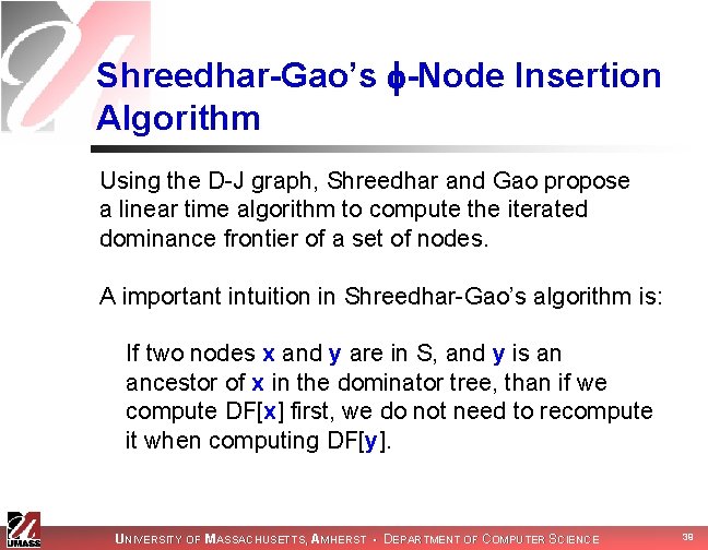
Shreedhar-Gao’s -Node Insertion Algorithm Using the D-J graph, Shreedhar and Gao propose a linear time algorithm to compute the iterated dominance frontier of a set of nodes. A important intuition in Shreedhar-Gao’s algorithm is: If two nodes x and y are in S, and y is an ancestor of x in the dominator tree, than if we compute DF[x] first, we do not need to recompute it when computing DF[y]. UNIVERSITY OF MASSACHUSETTS, AMHERST • DEPARTMENT OF COMPUTER SCIENCE 39

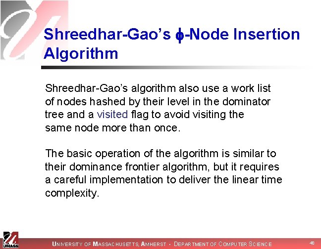
Shreedhar-Gao’s -Node Insertion Algorithm Shreedhar-Gao’s algorithm also use a work list of nodes hashed by their level in the dominator tree and a visited flag to avoid visiting the same node more than once. The basic operation of the algorithm is similar to their dominance frontier algorithm, but it requires a careful implementation to deliver the linear time complexity. UNIVERSITY OF MASSACHUSETTS, AMHERST • DEPARTMENT OF COMPUTER SCIENCE 40

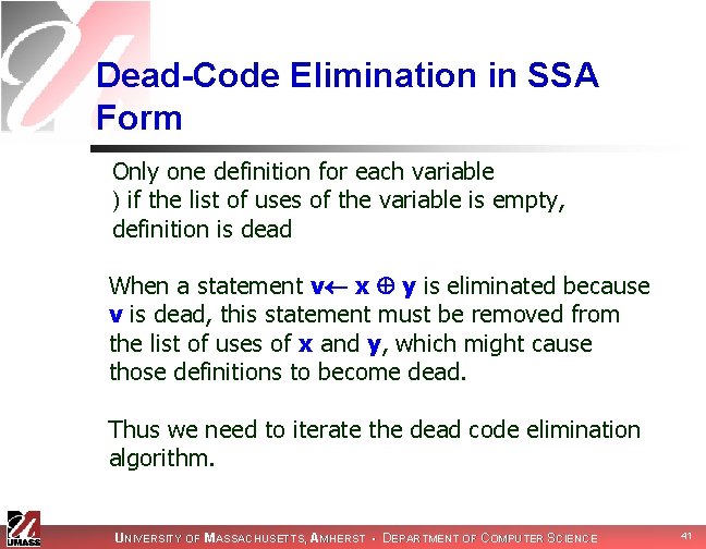
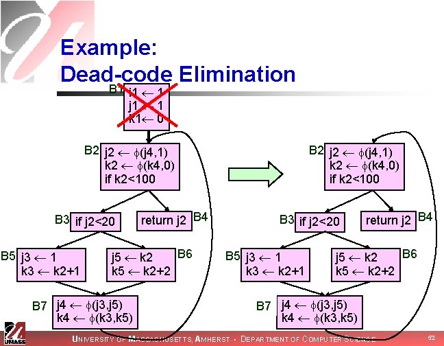
Dead-Code Elimination in SSA Form Only one definition for each variable ) if the list of uses of the variable is empty, definition is dead When a statement v x y is eliminated because v is dead, this statement must be removed from the list of uses of x and y, which might cause those definitions to become dead. Thus we need to iterate the dead code elimination algorithm. UNIVERSITY OF MASSACHUSETTS, AMHERST • DEPARTMENT OF COMPUTER SCIENCE 41

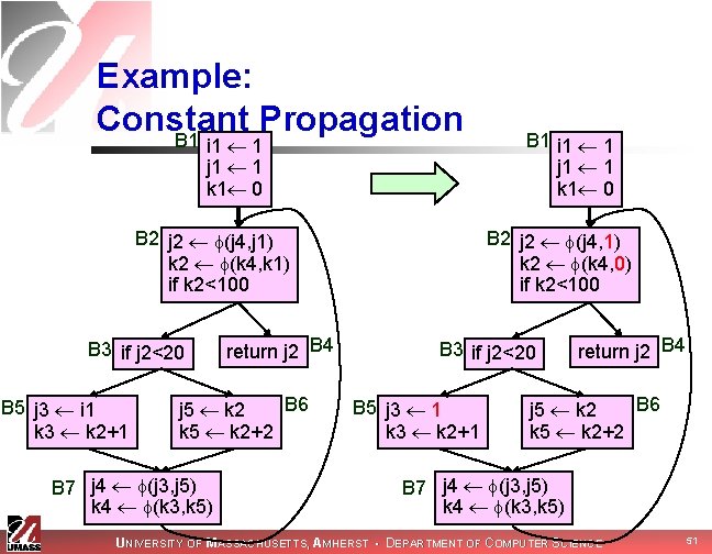
Simple Constant Propagation in SSA If there is a statement v c, where c is a constant, then all uses of v can be replaced for c. A function of the form v (c 1, c 2, …, cn) where all ci are identical can be replaced for v c. Using a work list algorithm in a program in SSA form, we can perform constant propagation in linear time In the next slide we assume that x, y, z are variables and a, b, c are constants. UNIVERSITY OF MASSACHUSETTS, AMHERST • DEPARTMENT OF COMPUTER SCIENCE 42

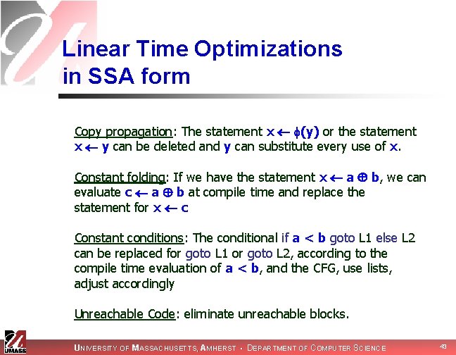
Linear Time Optimizations in SSA form Copy propagation: The statement x (y) or the statement x y can be deleted and y can substitute every use of x. Constant folding: If we have the statement x a b, we can evaluate c a b at compile time and replace the statement for x c Constant conditions: The conditional if a < b goto L 1 else L 2 can be replaced for goto L 1 or goto L 2, according to the compile time evaluation of a < b, and the CFG, use lists, adjust accordingly Unreachable Code: eliminate unreachable blocks. UNIVERSITY OF MASSACHUSETTS, AMHERST • DEPARTMENT OF COMPUTER SCIENCE 43

Next Time n Implementing other optimizations with SSA UNIVERSITY OF MASSACHUSETTS, AMHERST • DEPARTMENT OF COMPUTER SCIENCE 44

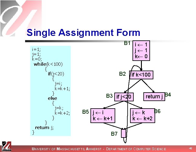
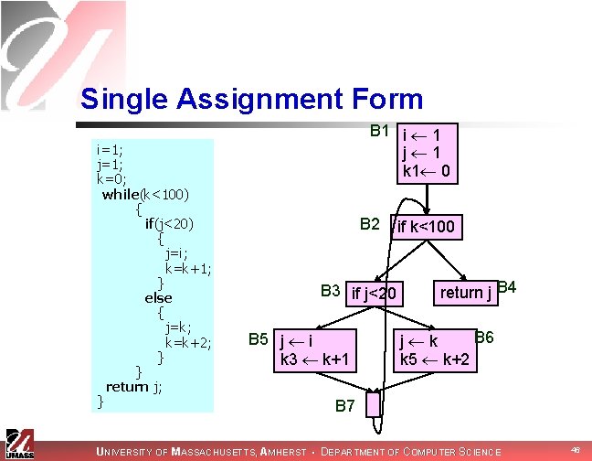
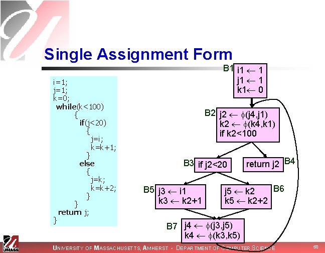
Single Assignment Form i=1; j=1; k=0; while(k<100) { if(j<20) { j=i; k=k+1; } else { j=k; k=k+2; } } return j; } B 1 i 1 j 1 k 0 B 2 B 3 if j<20 B 5 j i k k+1 if k<100 return j B 4 B 6 j k k k+2 B 7 UNIVERSITY OF MASSACHUSETTS, AMHERST • DEPARTMENT OF COMPUTER SCIENCE 45

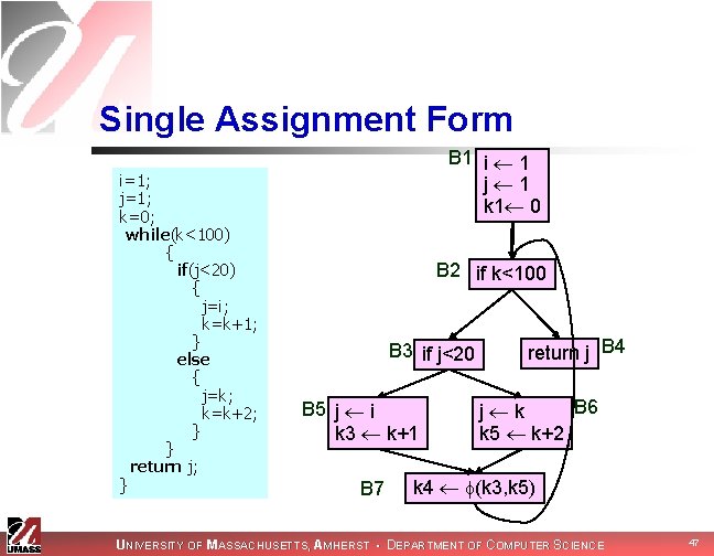
Single Assignment Form i=1; j=1; k=0; while(k<100) { if(j<20) { j=i; k=k+1; } else { j=k; k=k+2; } } return j; } B 1 i 1 j 1 k 1 0 B 2 B 3 if j<20 B 5 j i k 3 k+1 if k<100 return j B 4 B 6 j k k 5 k+2 B 7 UNIVERSITY OF MASSACHUSETTS, AMHERST • DEPARTMENT OF COMPUTER SCIENCE 46

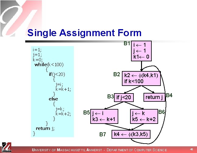
Single Assignment Form i=1; j=1; k=0; while(k<100) { if(j<20) { j=i; k=k+1; } else { j=k; k=k+2; } } return j; } B 1 i 1 j 1 k 1 0 B 2 if k<100 B 3 if j<20 B 5 j i k 3 k+1 B 7 return j B 4 B 6 j k k 5 k+2 k 4 (k 3, k 5) UNIVERSITY OF MASSACHUSETTS, AMHERST • DEPARTMENT OF COMPUTER SCIENCE 47

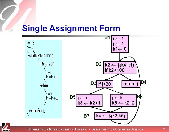
Single Assignment Form i=1; j=1; k=0; while(k<100) { if(j<20) { j=i; k=k+1; } else { j=k; k=k+2; } } return j; } B 1 i 1 j 1 k 1 0 B 2 k 2 (k 4, k 1) if k<100 B 3 if j<20 B 5 j i k 3 k+1 B 7 return j B 4 B 6 j k k 5 k+2 k 4 (k 3, k 5) UNIVERSITY OF MASSACHUSETTS, AMHERST • DEPARTMENT OF COMPUTER SCIENCE 48

Single Assignment Form i=1; j=1; k=0; while(k<100) { if(j<20) { j=i; k=k+1; } else { j=k; k=k+2; } } return j; } B 1 i 1 j 1 k 1 0 B 2 k 2 (k 4, k 1) if k 2<100 B 3 if j<20 B 5 j i k 3 k 2+1 B 7 return j B 4 B 6 j k k 5 k 2+2 k 4 (k 3, k 5) UNIVERSITY OF MASSACHUSETTS, AMHERST • DEPARTMENT OF COMPUTER SCIENCE 49

Single Assignment Form i=1; j=1; k=0; while(k<100) { if(j<20) { j=i; k=k+1; } else { j=k; k=k+2; } } return j; } B 1 i 1 1 j 1 1 k 1 0 B 2 j 2 (j 4, j 1) k 2 (k 4, k 1) if k 2<100 B 3 if j 2<20 B 5 j 3 i 1 k 3 k 2+1 return j 2 B 4 B 6 j 5 k 2 k 5 k 2+2 B 7 j 4 (j 3, j 5) k 4 (k 3, k 5) UNIVERSITY OF MASSACHUSETTS, AMHERST • DEPARTMENT OF COMPUTER SCIENCE 50

Example: Constant Propagation B 1 i 1 1 j 1 1 k 1 0 B 2 j 2 (j 4, j 1) k 2 (k 4, k 1) if k 2<100 B 3 if j 2<20 B 5 j 3 i 1 k 3 k 2+1 return j 2 B 4 B 6 j 5 k 2 k 5 k 2+2 B 7 j 4 (j 3, j 5) k 4 (k 3, k 5) B 1 i 1 1 j 1 1 k 1 0 B 2 j 2 (j 4, 1) k 2 (k 4, 0) if k 2<100 B 3 if j 2<20 B 5 j 3 1 k 3 k 2+1 return j 2 B 4 B 6 j 5 k 2 k 5 k 2+2 B 7 j 4 (j 3, j 5) k 4 (k 3, k 5) UNIVERSITY OF MASSACHUSETTS, AMHERST • DEPARTMENT OF COMPUTER SCIENCE 51

Example: Dead-code Elimination B 1 i 1 1 j 1 1 k 1 0 B 2 j 2 (j 4, 1) k 2 (k 4, 0) if k 2<100 B 3 if j 2<20 B 5 j 3 1 k 3 k 2+1 return j 2 B 4 B 6 j 5 k 2 k 5 k 2+2 B 7 j 4 (j 3, j 5) k 4 (k 3, k 5) UNIVERSITY OF MASSACHUSETTS, AMHERST • DEPARTMENT OF COMPUTER SCIENCE 52

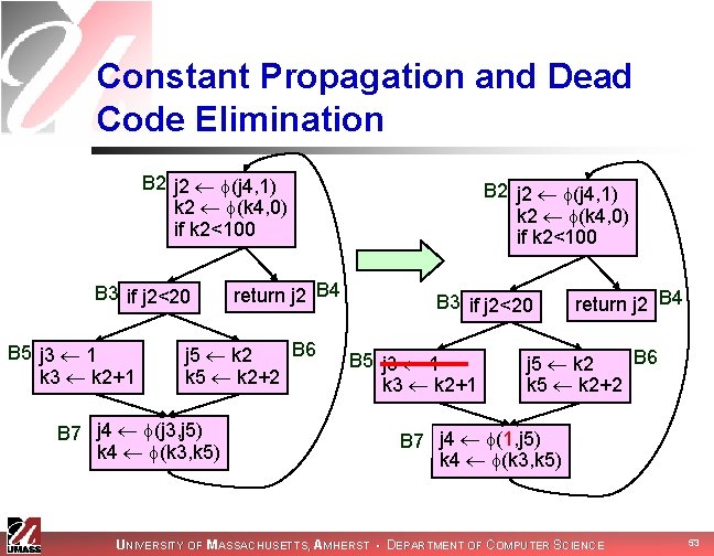
Constant Propagation and Dead Code Elimination B 2 j 2 (j 4, 1) k 2 (k 4, 0) if k 2<100 B 3 if j 2<20 B 5 j 3 1 k 3 k 2+1 return j 2 B 4 B 6 j 5 k 2 k 5 k 2+2 B 7 j 4 (j 3, j 5) k 4 (k 3, k 5) B 2 j 2 (j 4, 1) k 2 (k 4, 0) if k 2<100 B 3 if j 2<20 B 5 j 3 1 k 3 k 2+1 return j 2 B 4 B 6 j 5 k 2 k 5 k 2+2 B 7 j 4 (1, j 5) k 4 (k 3, k 5) UNIVERSITY OF MASSACHUSETTS, AMHERST • DEPARTMENT OF COMPUTER SCIENCE 53

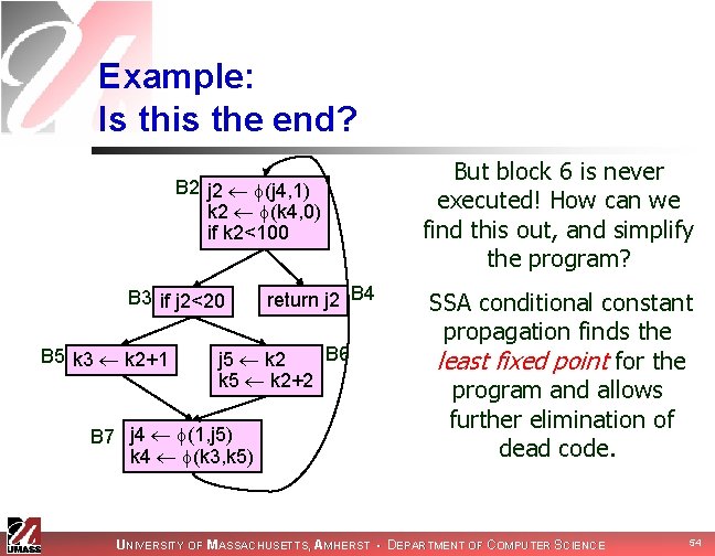
Example: Is this the end? B 2 j 2 (j 4, 1) k 2 (k 4, 0) if k 2<100 B 3 if j 2<20 B 5 k 3 k 2+1 return j 2 B 4 B 6 j 5 k 2 k 5 k 2+2 B 7 j 4 (1, j 5) k 4 (k 3, k 5) But block 6 is never executed! How can we find this out, and simplify the program? SSA conditional constant propagation finds the least fixed point for the program and allows further elimination of dead code. UNIVERSITY OF MASSACHUSETTS, AMHERST • DEPARTMENT OF COMPUTER SCIENCE 54

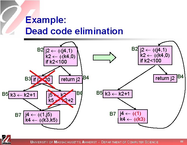
Example: Dead code elimination B 2 j 2 (j 4, 1) k 2 (k 4, 0) if k 2<100 B 3 if j 2<20 B 5 k 3 k 2+1 B 6 j 5 k 2 k 5 k 2+2 B 7 j 4 (1, j 5) k 4 (k 3, k 5) return j 2 B 4 B 5 k 3 k 2+1 B 7 j 4 (1) k 4 (k 3) UNIVERSITY OF MASSACHUSETTS, AMHERST • DEPARTMENT OF COMPUTER SCIENCE 55

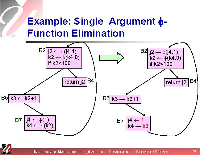
Example: Single Argument Function Elimination B 2 j 2 (j 4, 1) k 2 (k 4, 0) if k 2<100 return j 2 B 4 B 5 k 3 k 2+1 B 7 j 4 (1) k 4 (k 3) return j 2 B 4 B 5 k 3 k 2+1 B 7 j 4 1 k 4 k 3 UNIVERSITY OF MASSACHUSETTS, AMHERST • DEPARTMENT OF COMPUTER SCIENCE 56

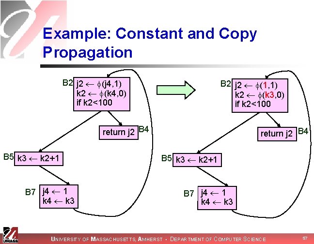
Example: Constant and Copy Propagation B 2 j 2 (j 4, 1) k 2 (k 4, 0) if k 2<100 B 2 j 2 (1, 1) k 2 (k 3, 0) if k 2<100 return j 2 B 4 B 5 k 3 k 2+1 B 7 j 4 1 k 4 k 3 UNIVERSITY OF MASSACHUSETTS, AMHERST • DEPARTMENT OF COMPUTER SCIENCE 57

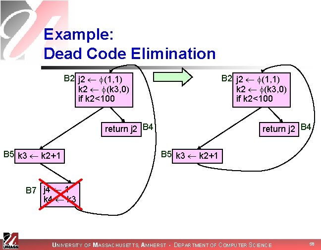
Example: Dead Code Elimination B 2 j 2 (1, 1) k 2 (k 3, 0) if k 2<100 return j 2 B 4 B 5 k 3 k 2+1 B 7 j 4 1 k 4 k 3 UNIVERSITY OF MASSACHUSETTS, AMHERST • DEPARTMENT OF COMPUTER SCIENCE 58

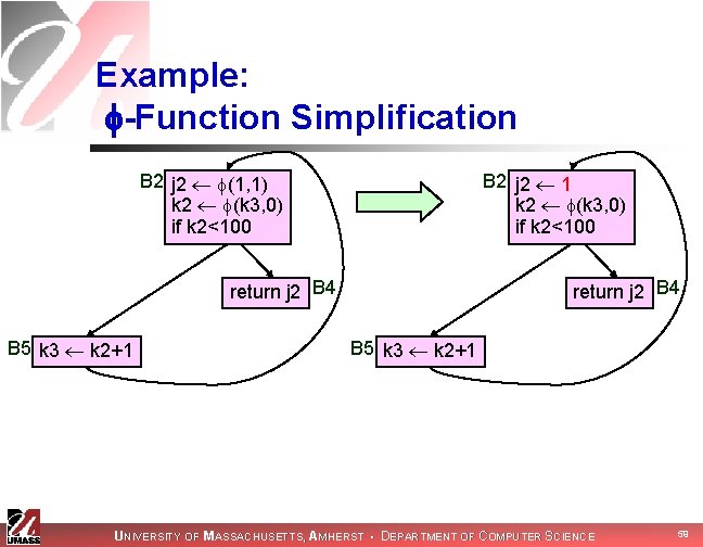
Example: -Function Simplification B 2 j 2 (1, 1) k 2 (k 3, 0) if k 2<100 B 2 j 2 1 k 2 (k 3, 0) if k 2<100 return j 2 B 4 B 5 k 3 k 2+1 UNIVERSITY OF MASSACHUSETTS, AMHERST • DEPARTMENT OF COMPUTER SCIENCE 59

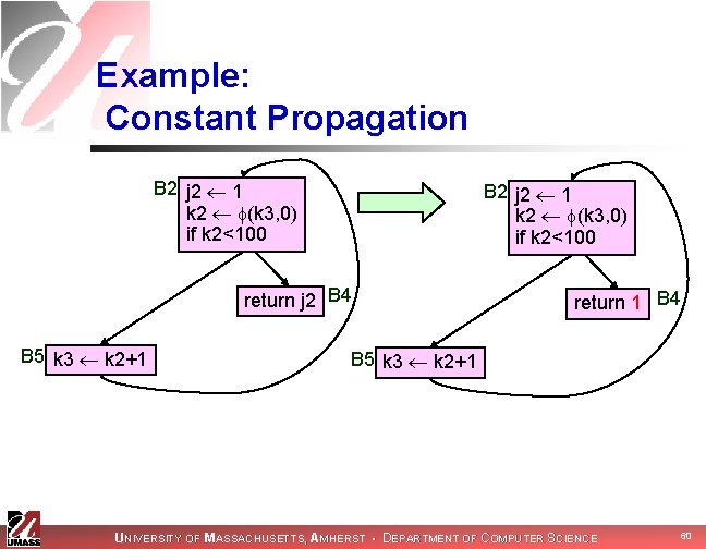
Example: Constant Propagation B 2 j 2 1 k 2 (k 3, 0) if k 2<100 return j 2 B 4 B 5 k 3 k 2+1 return 1 B 4 B 5 k 3 k 2+1 UNIVERSITY OF MASSACHUSETTS, AMHERST • DEPARTMENT OF COMPUTER SCIENCE 60

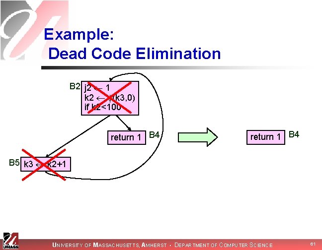
Example: Dead Code Elimination B 2 j 2 1 k 2 (k 3, 0) if k 2<100 return 1 B 4 B 5 k 3 k 2+1 UNIVERSITY OF MASSACHUSETTS, AMHERST • DEPARTMENT OF COMPUTER SCIENCE 61

Next Time UNIVERSITY OF MASSACHUSETTS, AMHERST • DEPARTMENT OF COMPUTER SCIENCE 62