Stats 330 Lecture 20 Department of Statistics 2012

Stats 330: Lecture 20 © Department of Statistics 2012 STATS 330 Lecture 20: Slide 1

Categorical responses • Up until now, we have always assumed that our response variable is continuous. • For the rest of the course, we will discuss models for categorical or count responses. • Eg – alive/dead (binary response as a function of risk factors for heart disease) – count traffic past a fixed point in 1 hour (count response as function of day of week, time of day, weather conditions) © Department of Statistics 2012 STATS 330 Lecture 20: Slide 2

Categorical responses (cont) • In the first part of the course, we modelled continuous responses using the normal distribution. • We assumed that the response was normal with a mean depending on the explanatory variables. • For categorical responses, we do something similar: – If the response is binary (y/N, 0/1, alive/dead), or a proportion, we use the binomial distribution – If the response is a count, we use the Poisson distribution • As before, we let the means of these distributions depend on the explanatory variables. © Department of Statistics 2012 STATS 330 Lecture 20: Slide 3

Plan of action • For the next few lectures, we concentrate on the first case, where the response is binary, or a proportion. • Then we will move on to the analysis of count data, including the analysis of contingency tables. © Department of Statistics 2012 STATS 330 Lecture 20: Slide 4

Binary data: example • The prevalence of coronary heart disease (CHD) depends very much on age: the probability that a person randomly chosen from a population is suffering from CHD depends on the age of the person (and on lots of other factors as well, such as smoking history, diet, exercise and so on). © Department of Statistics 2012 STATS 330 Lecture 20: Slide 5

CHD data The data on the next slide were collected during a medical study. A sample of individuals was selected at random, and their age and CHD status was recorded. There are 2 variables AGE: age in years (continuous variable) CHD: 0=no CHD, 1=CHD (binary variable) © Department of Statistics 2012 STATS 330 Lecture 20: Slide 6

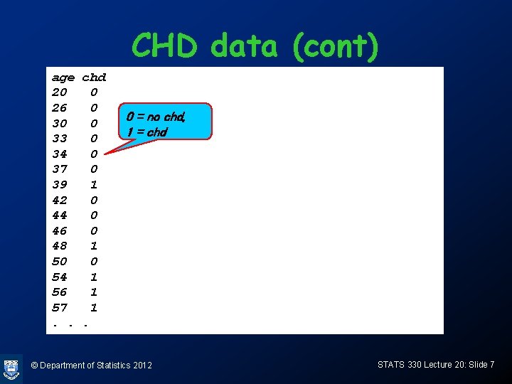
CHD data (cont) age chd 20 0 26 0 30 0 33 0 34 0 37 0 39 1 42 0 44 0 46 0 48 1 50 0 54 1 56 1 57 1. . . 0 = no chd, 1 = chd © Department of Statistics 2012 STATS 330 Lecture 20: Slide 7

Plot of the data plot(age, chd) © Department of Statistics 2012 STATS 330 Lecture 20: Slide 8

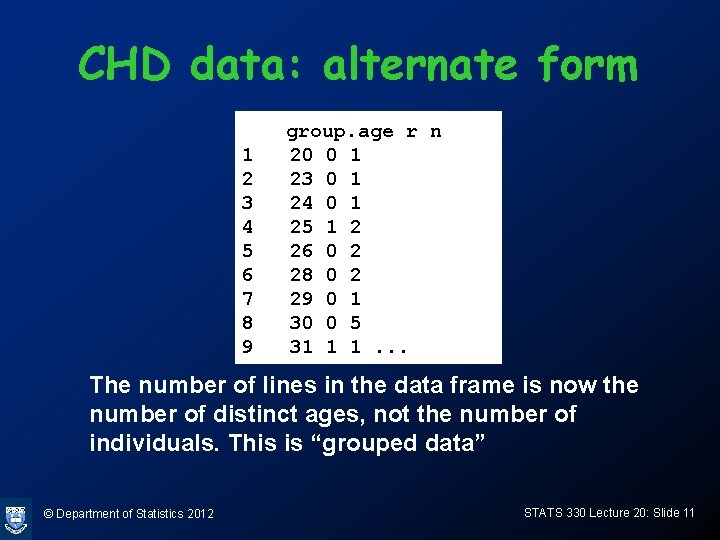
Ungrouped and grouped data • In the data set on the previous slide, every line of the data file corresponds to an individual in the sample. This is called ungrouped data • If there are many identical ages, a more compact way of representing the data is as “grouped data” © Department of Statistics 2012 STATS 330 Lecture 20: Slide 9

CHD data (cont) > attach(chd. df) > sorted. chd. df<-chd. df[order(age), ] > sorted. chd. df age chd Alternate way of entering the same data: record 1 20 0 2 23 0 (i) the number of times (n) each age occurs 3 24 0 4 25 0 (repeat counts) 5 25 1 6 26 0 (i) The number of persons (r) of that age having 7 26 0 CHD 8 28 0 9 28 0 (CHD counts) 10 29 0 11 30 0 i. e. age 30 occurs 5 times with all 5 persons not 12 30 0 having CHD 13 30 0 14 30 0 Hence, r = 0 and n = 5 15 30 0 16 31 1 © Department of Statistics 2012 STATS 330 Lecture 20: Slide 10

CHD data: alternate form 1 2 3 4 5 6 7 8 9 group. age r n 20 0 1 23 0 1 24 0 1 25 1 2 26 0 2 28 0 2 29 0 1 30 0 5 31 1 1. . . The number of lines in the data frame is now the number of distinct ages, not the number of individuals. This is “grouped data” © Department of Statistics 2012 STATS 330 Lecture 20: Slide 11

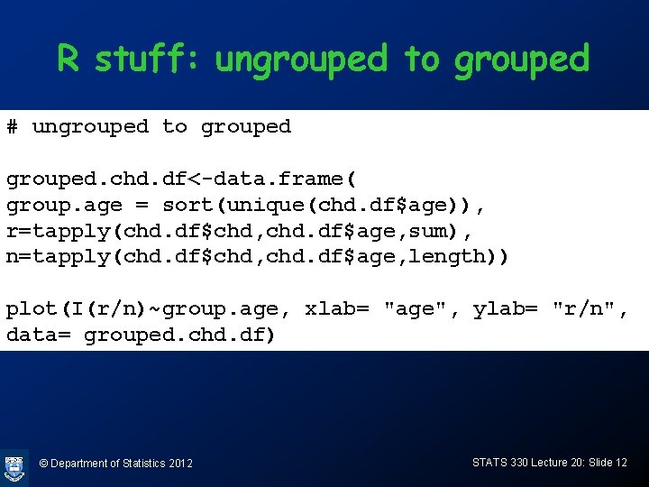
R stuff: ungrouped to grouped # ungrouped to grouped. chd. df<-data. frame( group. age = sort(unique(chd. df$age)), r=tapply(chd. df$chd, chd. df$age, sum), n=tapply(chd. df$chd, chd. df$age, length)) plot(I(r/n)~group. age, xlab= "age", ylab= "r/n", data= grouped. chd. df) © Department of Statistics 2012 STATS 330 Lecture 20: Slide 12

© Department of Statistics 2012 STATS 330 Lecture 20: Slide 13

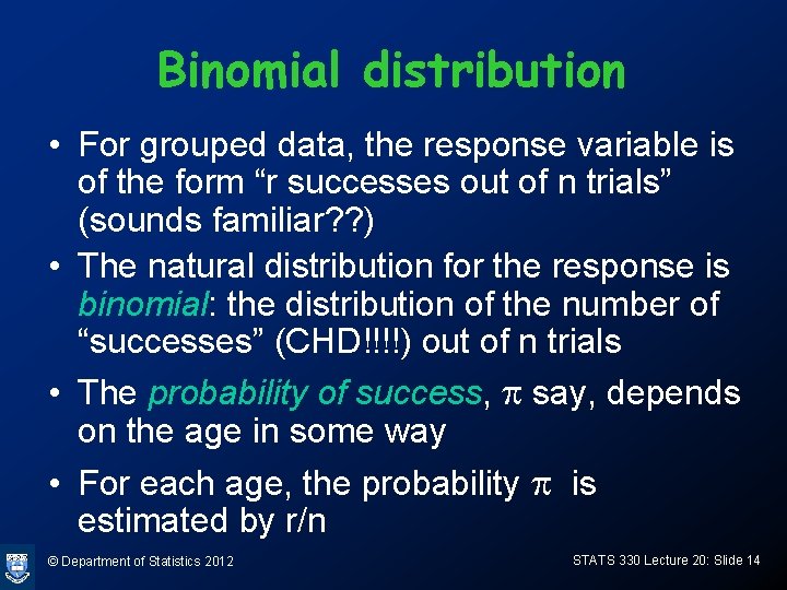
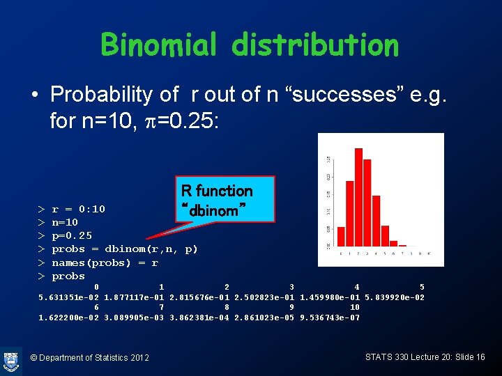
Binomial distribution • For grouped data, the response variable is of the form “r successes out of n trials” (sounds familiar? ? ) • The natural distribution for the response is binomial: the distribution of the number of “successes” (CHD!!!!) out of n trials • The probability of success, p say, depends on the age in some way • For each age, the probability p is estimated by r/n © Department of Statistics 2012 STATS 330 Lecture 20: Slide 14

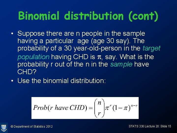
Binomial distribution (cont) • Suppose there are n people in the sample having a particular age (age 30 say). The probability of a 30 year-old-person in the target population having CHD is p, say. What is the probability r out of the n in the sample have CHD? • Use the binomial distribution: © Department of Statistics 2012 STATS 330 Lecture 20: Slide 15

Binomial distribution • Probability of r out of n “successes” e. g. for n=10, p=0. 25: > > > R function “dbinom” r = 0: 10 n=10 p=0. 25 probs = dbinom(r, n, p) names(probs) = r probs 0 1 2 3 4 5 5. 631351 e-02 1. 877117 e-01 2. 815676 e-01 2. 502823 e-01 1. 459980 e-01 5. 839920 e-02 6 7 8 9 10 1. 622200 e-02 3. 089905 e-03 3. 862381 e-04 2. 861023 e-05 9. 536743 e-07 © Department of Statistics 2012 STATS 330 Lecture 20: Slide 16

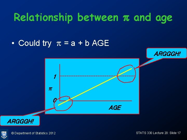
Relationship between p and age • Could try p = a + b AGE ARGGGH! 1 p 0 AGE ARGGGH! © Department of Statistics 2012 STATS 330 Lecture 20: Slide 17

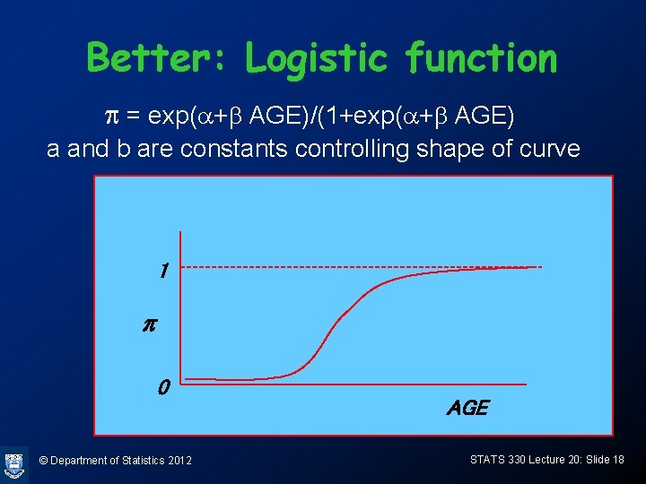
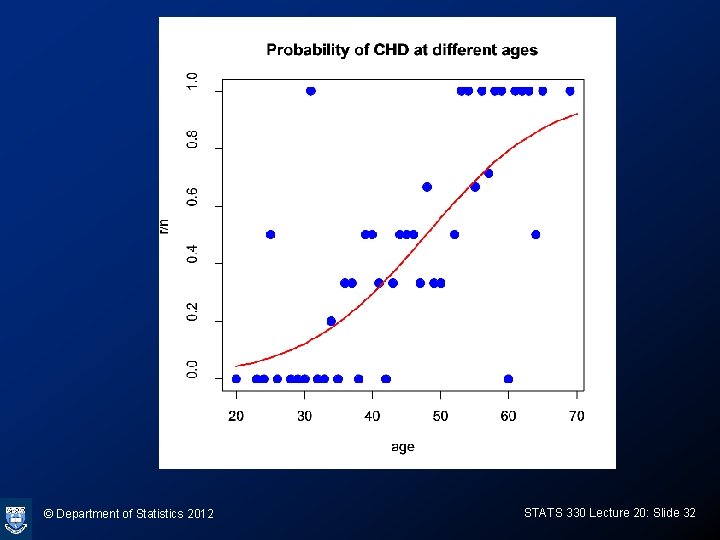
Better: Logistic function p = exp(a+b AGE)/(1+exp(a+b AGE) a and b are constants controlling shape of curve 1 p 0 © Department of Statistics 2012 AGE STATS 330 Lecture 20: Slide 18

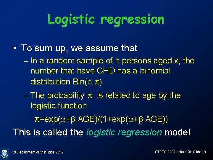
Logistic regression • To sum up, we assume that – In a random sample of n persons aged x, the number that have CHD has a binomial distribution Bin(n, p) – The probability p is related to age by the logistic function p=exp(a+b AGE)/(1+exp(a+b AGE)) This is called the logistic regression model © Department of Statistics 2012 STATS 330 Lecture 20: Slide 19

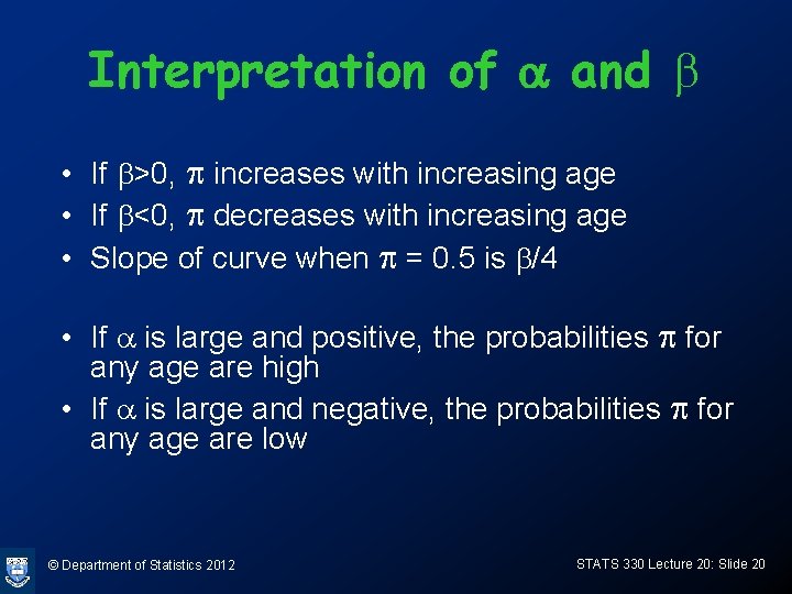
Interpretation of a and b • If b>0, p increases with increasing age • If b<0, p decreases with increasing age • Slope of curve when p = 0. 5 is b/4 • If a is large and positive, the probabilities p for any age are high • If a is large and negative, the probabilities p for any age are low © Department of Statistics 2012 STATS 330 Lecture 20: Slide 20

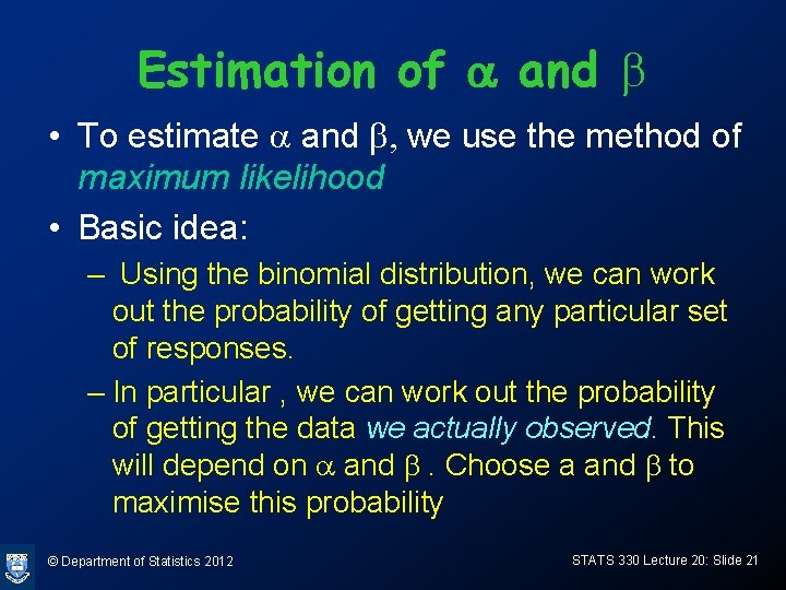
Estimation of a and b • To estimate a and b, we use the method of maximum likelihood • Basic idea: – Using the binomial distribution, we can work out the probability of getting any particular set of responses. – In particular , we can work out the probability of getting the data we actually observed. This will depend on a and b. Choose a and b to maximise this probability © Department of Statistics 2012 STATS 330 Lecture 20: Slide 21

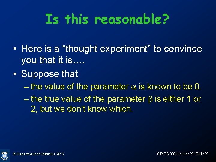
Is this reasonable? • Here is a “thought experiment” to convince you that it is…. • Suppose that – the value of the parameter a is known to be 0. – the true value of the parameter b is either 1 or 2, but we don’t know which. © Department of Statistics 2012 STATS 330 Lecture 20: Slide 22

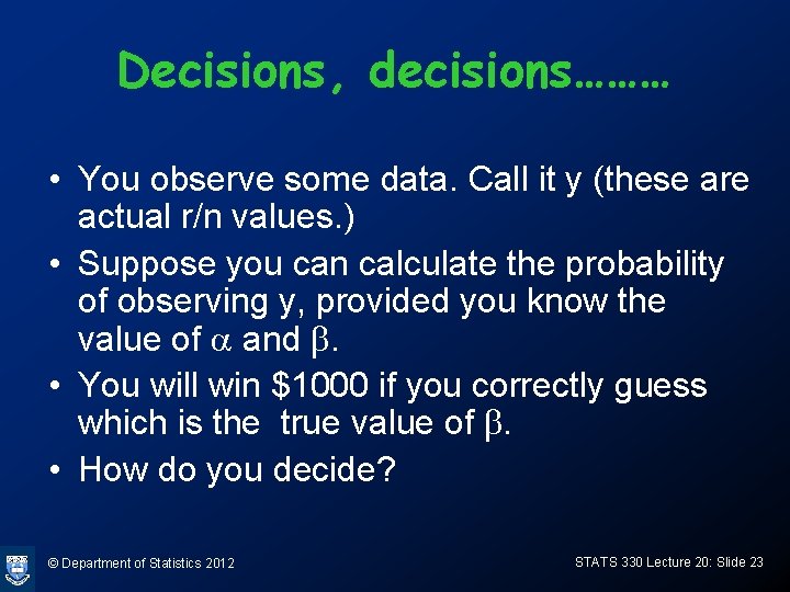
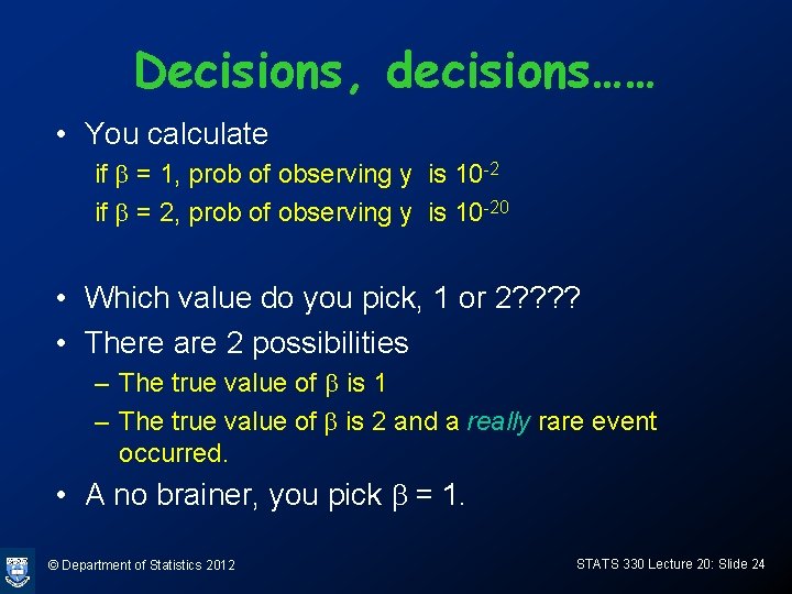
Decisions, decisions……… • You observe some data. Call it y (these are actual r/n values. ) • Suppose you can calculate the probability of observing y, provided you know the value of a and b. • You will win $1000 if you correctly guess which is the true value of b. • How do you decide? © Department of Statistics 2012 STATS 330 Lecture 20: Slide 23

Decisions, decisions…… • You calculate if b = 1, prob of observing y is 10 -2 if b = 2, prob of observing y is 10 -20 • Which value do you pick, 1 or 2? ? • There are 2 possibilities – The true value of b is 1 – The true value of b is 2 and a really rare event occurred. • A no brainer, you pick b = 1. © Department of Statistics 2012 STATS 330 Lecture 20: Slide 24

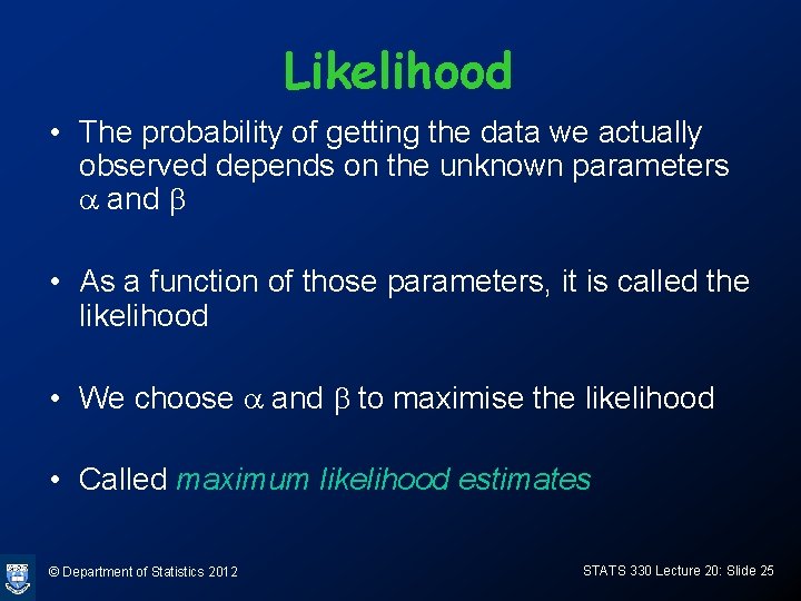
Likelihood • The probability of getting the data we actually observed depends on the unknown parameters a and b • As a function of those parameters, it is called the likelihood • We choose a and b to maximise the likelihood • Called maximum likelihood estimates © Department of Statistics 2012 STATS 330 Lecture 20: Slide 25

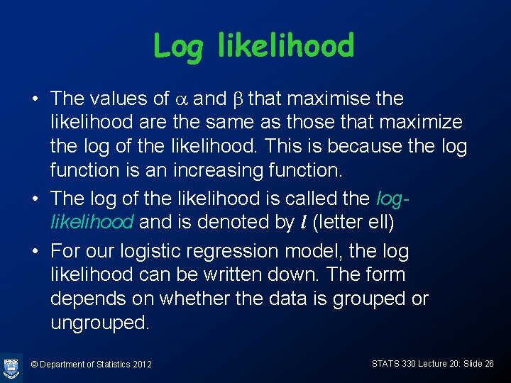
Log likelihood • The values of a and b that maximise the likelihood are the same as those that maximize the log of the likelihood. This is because the log function is an increasing function. • The log of the likelihood is called the loglikelihood and is denoted by l (letter ell) • For our logistic regression model, the log likelihood can be written down. The form depends on whether the data is grouped or ungrouped. © Department of Statistics 2012 STATS 330 Lecture 20: Slide 26

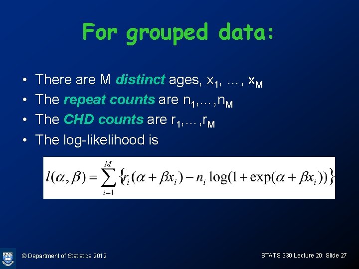
For grouped data: • • There are M distinct ages, x 1, …, x. M The repeat counts are n 1, …, n. M The CHD counts are r 1, …, r. M The log-likelihood is © Department of Statistics 2012 STATS 330 Lecture 20: Slide 27

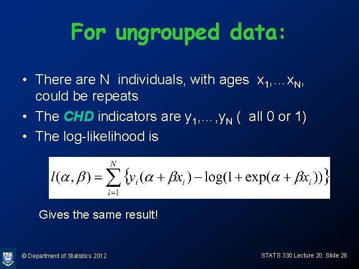
For ungrouped data: • There are N individuals, with ages x 1, …x. N, could be repeats • The CHD indicators are y 1, …, y. N ( all 0 or 1) • The log-likelihood is Gives the same result! © Department of Statistics 2012 STATS 330 Lecture 20: Slide 28

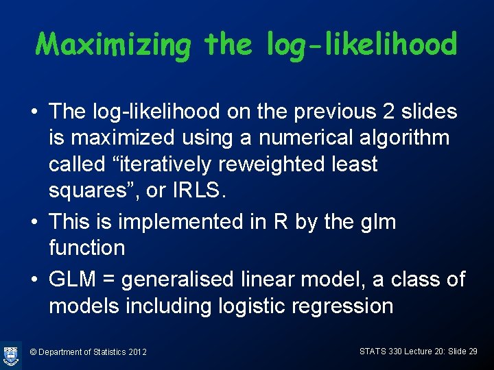
Maximizing the log-likelihood • The log-likelihood on the previous 2 slides is maximized using a numerical algorithm called “iteratively reweighted least squares”, or IRLS. • This is implemented in R by the glm function • GLM = generalised linear model, a class of models including logistic regression © Department of Statistics 2012 STATS 330 Lecture 20: Slide 29

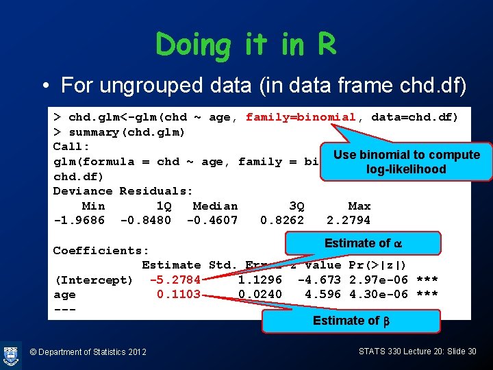
Doing it in R • For ungrouped data (in data frame chd. df) > chd. glm<-glm(chd ~ age, family=binomial, data=chd. df) > summary(chd. glm) Call: Use binomial to compute glm(formula = chd ~ age, family = binomial, data = log-likelihood chd. df) Deviance Residuals: Min 1 Q Median 3 Q Max -1. 9686 -0. 8480 -0. 4607 0. 8262 2. 2794 Estimate of a Coefficients: Estimate Std. Error z value Pr(>|z|) (Intercept) -5. 2784 1. 1296 -4. 673 2. 97 e-06 *** age 0. 1103 0. 0240 4. 596 4. 30 e-06 *** --Estimate of b © Department of Statistics 2012 STATS 330 Lecture 20: Slide 30

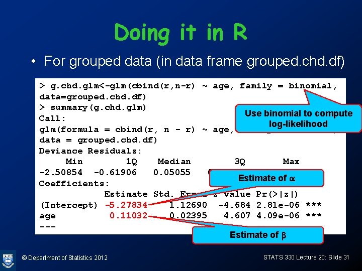
Doing it in R • For grouped data (in data frame grouped. chd. df) > g. chd. glm<-glm(cbind(r, n-r) ~ age, family = binomial, data=grouped. chd. df) > summary(g. chd. glm) Use binomial to compute Call: log-likelihood glm(formula = cbind(r, n - r) ~ age, family = binomial, data = grouped. chd. df) Deviance Residuals: Min 1 Q Median 3 Q Max -2. 50854 -0. 61906 0. 05055 0. 59488 2. 00167 Estimate of a Coefficients: Estimate Std. Error z value Pr(>|z|) (Intercept) -5. 27834 1. 12690 -4. 684 2. 81 e-06 *** age 0. 11032 0. 02395 4. 607 4. 09 e-06 *** --Estimate of b © Department of Statistics 2012 STATS 330 Lecture 20: Slide 31

© Department of Statistics 2012 STATS 330 Lecture 20: Slide 32

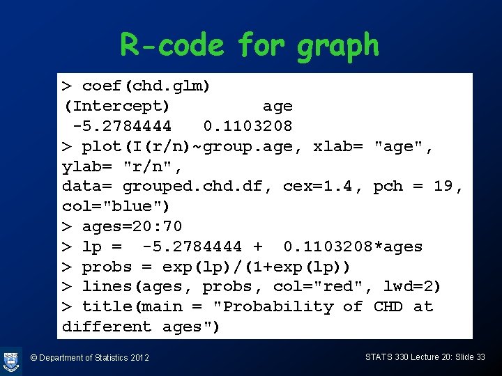
R-code for graph > coef(chd. glm) (Intercept) age -5. 2784444 0. 1103208 > plot(I(r/n)~group. age, xlab= "age", ylab= "r/n", data= grouped. chd. df, cex=1. 4, pch = 19, col="blue") > ages=20: 70 > lp = -5. 2784444 + 0. 1103208*ages > probs = exp(lp)/(1+exp(lp)) > lines(ages, probs, col="red", lwd=2) > title(main = "Probability of CHD at different ages") © Department of Statistics 2012 STATS 330 Lecture 20: Slide 33