STATS 330 Lecture 17 9182020 330 lecture 17

STATS 330: Lecture 17 9/18/2020 330 lecture 17 1

Factors § In the models discussed so far, all explanatory variables have been numeric § Now we want to incorporate categorical variables into our models § In R, categorical variables are called factors 9/18/2020 330 lecture 17 2

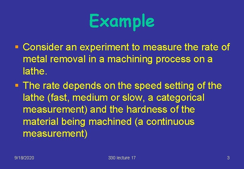
Example § Consider an experiment to measure the rate of metal removal in a machining process on a lathe. § The rate depends on the speed setting of the lathe (fast, medium or slow, a categorical measurement) and the hardness of the material being machined (a continuous measurement) 9/18/2020 330 lecture 17 3

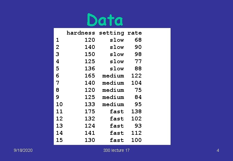
Data 1 2 3 4 5 6 7 8 9 10 11 12 13 14 15 9/18/2020 hardness setting rate 120 slow 68 140 slow 90 150 slow 98 125 slow 77 136 slow 88 165 medium 122 140 medium 104 120 medium 75 125 medium 84 133 medium 95 175 fast 138 132 fast 102 124 fast 93 141 fast 112 130 fast 100 330 lecture 17 4

9/18/2020 330 lecture 17 5

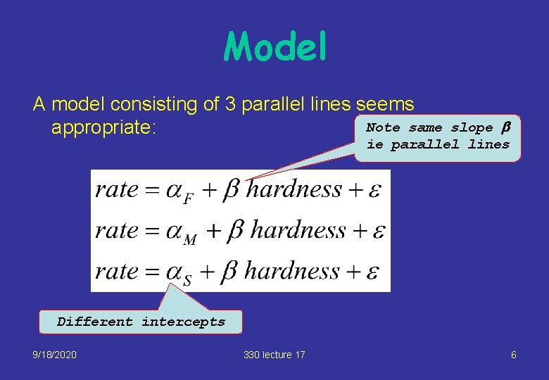
Model A model consisting of 3 parallel lines seems Note same appropriate: slope b ie parallel lines Different intercepts 9/18/2020 330 lecture 17 6

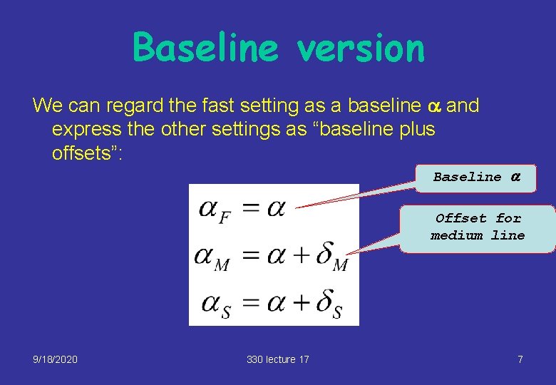
Baseline version We can regard the fast setting as a baseline a and express the other settings as “baseline plus offsets”: Baseline a Offset for medium line 9/18/2020 330 lecture 17 7

Baseline version (2) We can then write the model as 9/18/2020 330 lecture 17 8

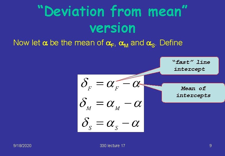
“Deviation from mean” version Now let a be the mean of a. F, a. M and a. S. Define “fast” line intercept Mean of intercepts 9/18/2020 330 lecture 17 9

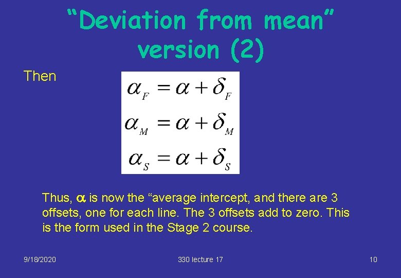
“Deviation from mean” version (2) Then Thus, a is now the “average intercept, and there are 3 offsets, one for each line. The 3 offsets add to zero. This is the form used in the Stage 2 course. 9/18/2020 330 lecture 17 10

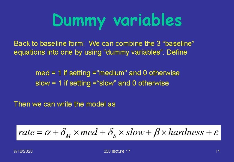
Dummy variables Back to baseline form: We can combine the 3 “baseline” equations into one by using “dummy variables”. Define med = 1 if setting =“medium” and 0 otherwise slow = 1 if setting =“slow” and 0 otherwise Then we can write the model as 9/18/2020 330 lecture 17 11

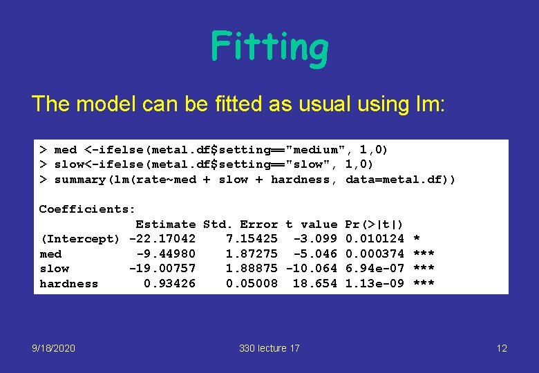
Fitting The model can be fitted as usual using lm: > med <-ifelse(metal. df$setting=="medium", 1, 0) > slow<-ifelse(metal. df$setting=="slow", 1, 0) > summary(lm(rate~med + slow + hardness, data=metal. df)) Coefficients: Estimate Std. Error t value Pr(>|t|) (Intercept) -22. 17042 7. 15425 -3. 099 0. 010124 * med -9. 44980 1. 87275 -5. 046 0. 000374 *** slow -19. 00757 1. 88875 -10. 064 6. 94 e-07 *** hardness 0. 93426 0. 05008 18. 654 1. 13 e-09 *** 9/18/2020 330 lecture 17 12

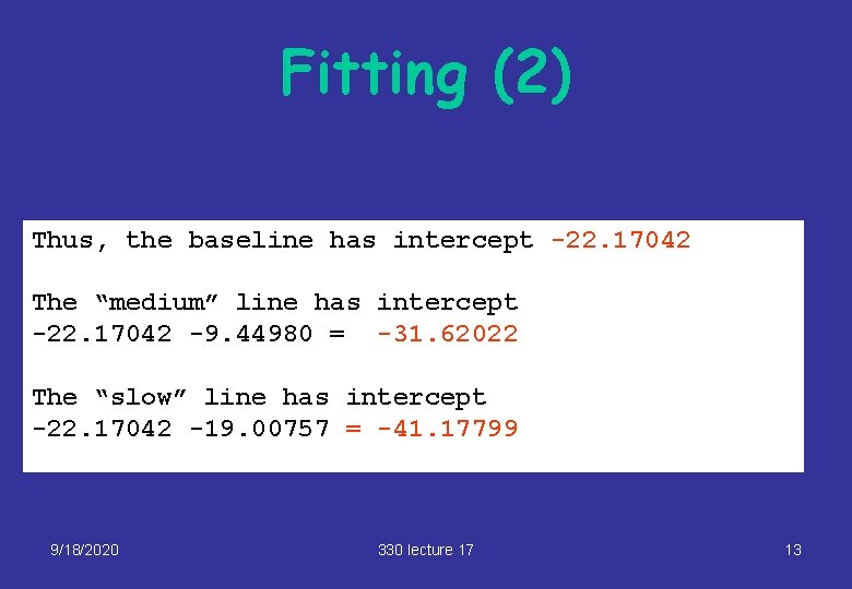
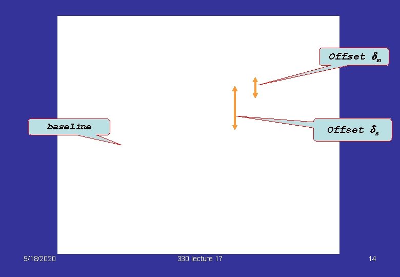
Fitting (2) Thus, the baseline has intercept -22. 17042 The “medium” line has intercept -22. 17042 -9. 44980 = -31. 62022 The “slow” line has intercept -22. 17042 -19. 00757 = -41. 17799 9/18/2020 330 lecture 17 13

Offset dm baseline 9/18/2020 Offset ds 330 lecture 17 14

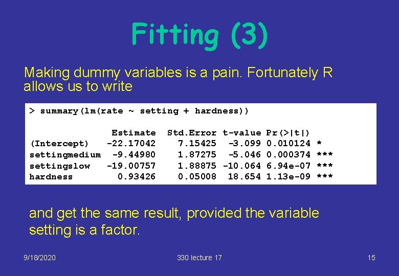
Fitting (3) Making dummy variables is a pain. Fortunately R allows us to write > summary(lm(rate ~ setting + hardness)) Estimate (Intercept) -22. 17042 settingmedium -9. 44980 settingslow -19. 00757 hardness 0. 93426 Std. Error t-value Pr(>|t|) 7. 15425 -3. 099 0. 010124 * 1. 87275 -5. 046 0. 000374 *** 1. 88875 -10. 064 6. 94 e-07 *** 0. 05008 18. 654 1. 13 e-09 *** and get the same result, provided the variable setting is a factor. 9/18/2020 330 lecture 17 15

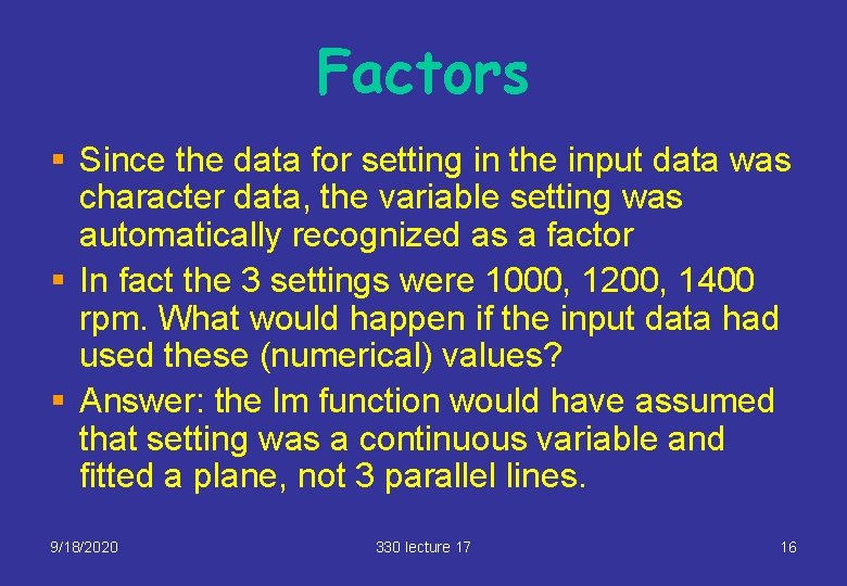
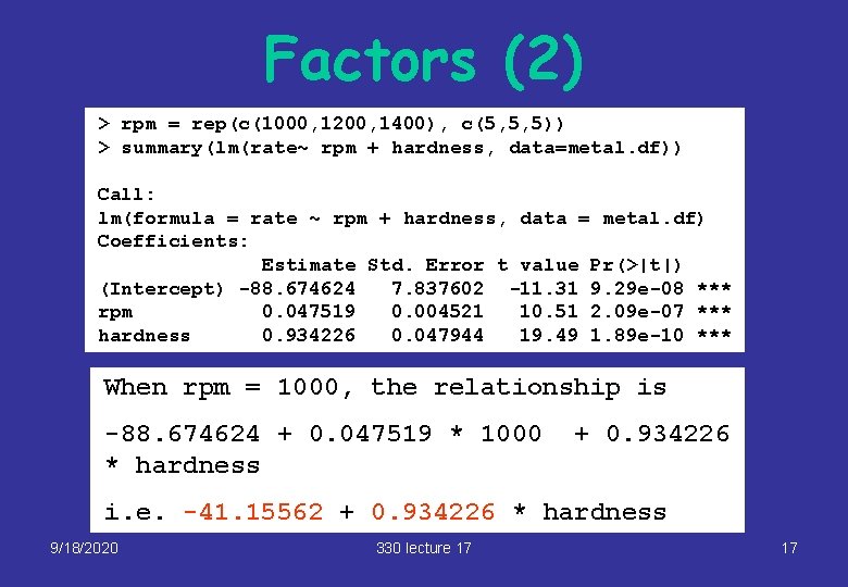
Factors § Since the data for setting in the input data was character data, the variable setting was automatically recognized as a factor § In fact the 3 settings were 1000, 1200, 1400 rpm. What would happen if the input data had used these (numerical) values? § Answer: the lm function would have assumed that setting was a continuous variable and fitted a plane, not 3 parallel lines. 9/18/2020 330 lecture 17 16

Factors (2) > rpm = rep(c(1000, 1200, 1400), c(5, 5, 5)) > summary(lm(rate~ rpm + hardness, data=metal. df)) Call: lm(formula = rate ~ rpm + hardness, data = metal. df) Coefficients: Estimate Std. Error t value Pr(>|t|) (Intercept) -88. 674624 7. 837602 -11. 31 9. 29 e-08 *** rpm 0. 047519 0. 004521 10. 51 2. 09 e-07 *** hardness 0. 934226 0. 047944 19. 49 1. 89 e-10 *** When rpm = 1000, the relationship is -88. 674624 + 0. 047519 * 1000 * hardness + 0. 934226 i. e. -41. 15562 + 0. 934226 * hardness 9/18/2020 330 lecture 17 17

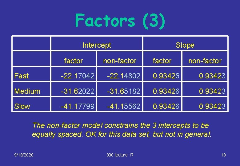
Factors (3) Intercept factor non-factor Slope factor non-factor Fast -22. 17042 -22. 14802 0. 93426 0. 93423 Medium -31. 62022 -31. 65182 0. 93426 0. 93423 Slow -41. 17799 -41. 15562 0. 93426 0. 93423 The non-factor model constrains the 3 intercepts to be equally spaced. OK for this data set, but not in general. 9/18/2020 330 lecture 17 18

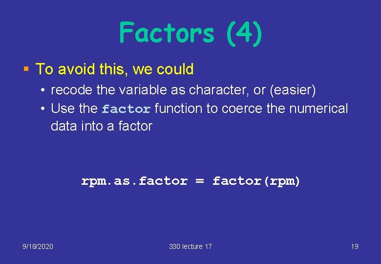
Factors (4) § To avoid this, we could • recode the variable as character, or (easier) • Use the factor function to coerce the numerical data into a factor rpm. as. factor = factor(rpm) 9/18/2020 330 lecture 17 19

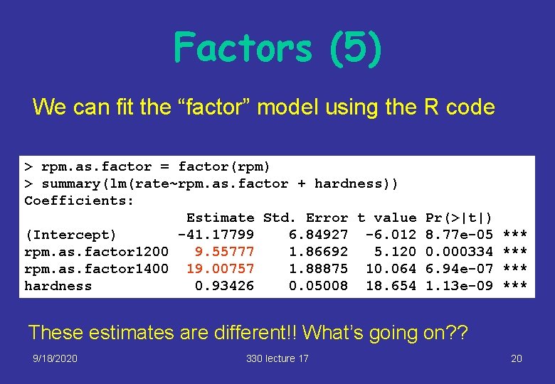
Factors (5) We can fit the “factor” model using the R code > rpm. as. factor = factor(rpm) > summary(lm(rate~rpm. as. factor + hardness)) Coefficients: Estimate Std. Error t value (Intercept) -41. 17799 6. 84927 -6. 012 rpm. as. factor 1200 9. 55777 1. 86692 5. 120 rpm. as. factor 1400 19. 00757 1. 88875 10. 064 hardness 0. 93426 0. 05008 18. 654 Pr(>|t|) 8. 77 e-05 0. 000334 6. 94 e-07 1. 13 e-09 *** *** These estimates are different!! What’s going on? ? 9/18/2020 330 lecture 17 20

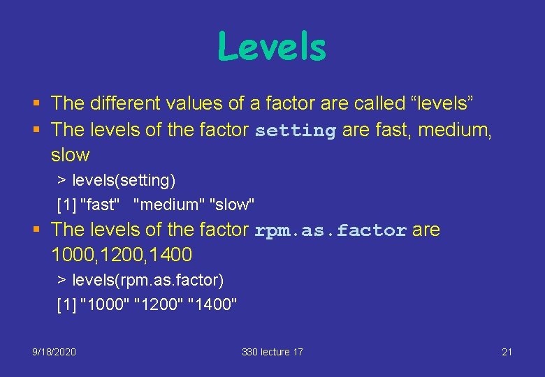
Levels § The different values of a factor are called “levels” § The levels of the factor setting are fast, medium, slow > levels(setting) [1] "fast" "medium" "slow" § The levels of the factor rpm. as. factor are 1000, 1200, 1400 > levels(rpm. as. factor) [1] "1000" "1200" "1400" 9/18/2020 330 lecture 17 21

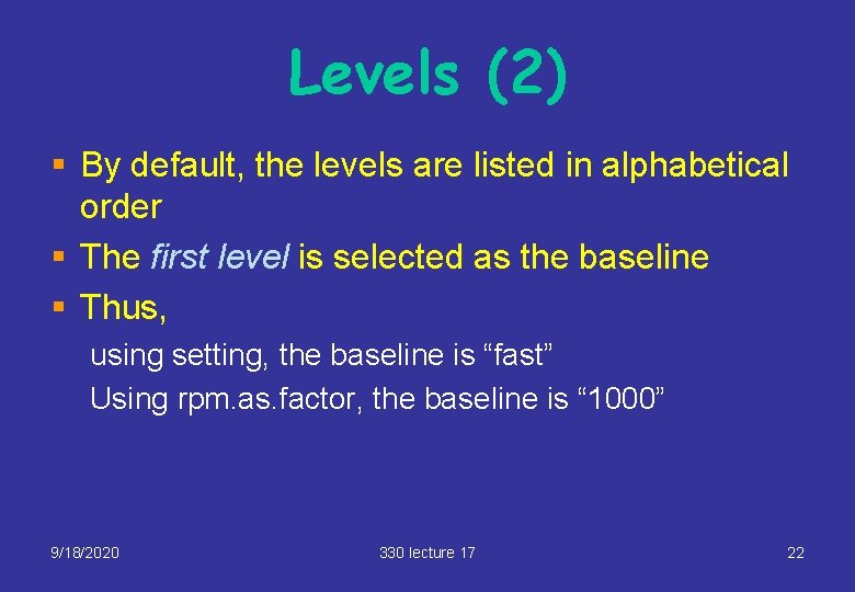
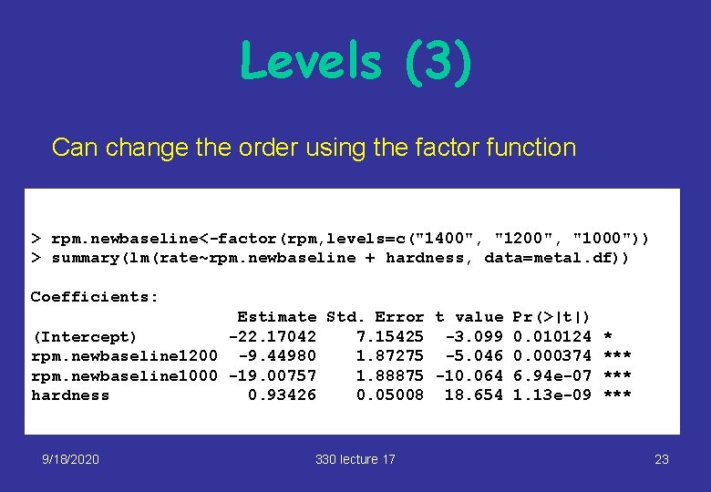
Levels (2) § By default, the levels are listed in alphabetical order § The first level is selected as the baseline § Thus, using setting, the baseline is “fast” Using rpm. as. factor, the baseline is “ 1000” 9/18/2020 330 lecture 17 22

Levels (3) Can change the order using the factor function > rpm. newbaseline<-factor(rpm, levels=c("1400", "1200", "1000")) > summary(lm(rate~rpm. newbaseline + hardness, data=metal. df)) Coefficients: Estimate Std. Error t value Pr(>|t|) (Intercept) -22. 17042 7. 15425 -3. 099 0. 010124 * rpm. newbaseline 1200 -9. 44980 1. 87275 -5. 046 0. 000374 *** rpm. newbaseline 1000 -19. 00757 1. 88875 -10. 064 6. 94 e-07 *** hardness 0. 93426 0. 05008 18. 654 1. 13 e-09 *** 9/18/2020 330 lecture 17 23

Non-parallel lines § What if the lines aren’t parallel? Then the betas are different: the model becomes 9/18/2020 330 lecture 17 24

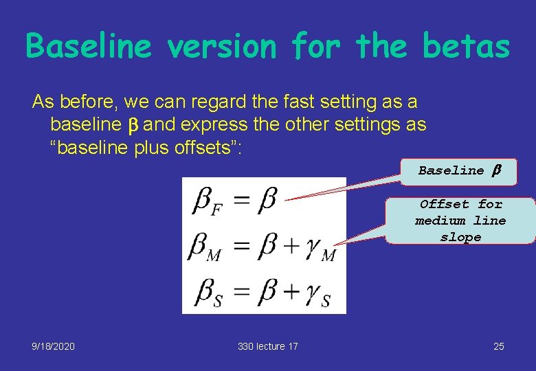
Baseline version for the betas As before, we can regard the fast setting as a baseline b and express the other settings as “baseline plus offsets”: Baseline b Offset for medium line slope 9/18/2020 330 lecture 17 25

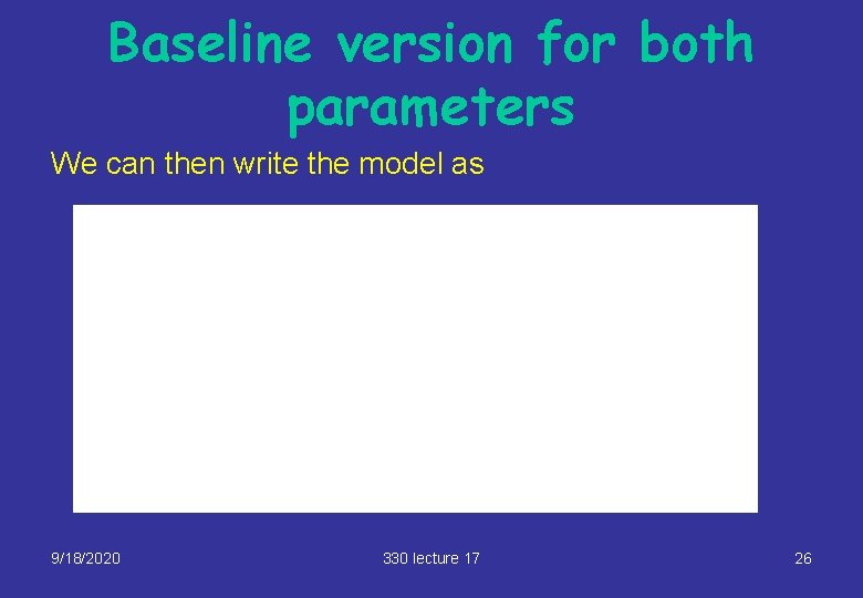
Baseline version for both parameters We can then write the model as 9/18/2020 330 lecture 17 26

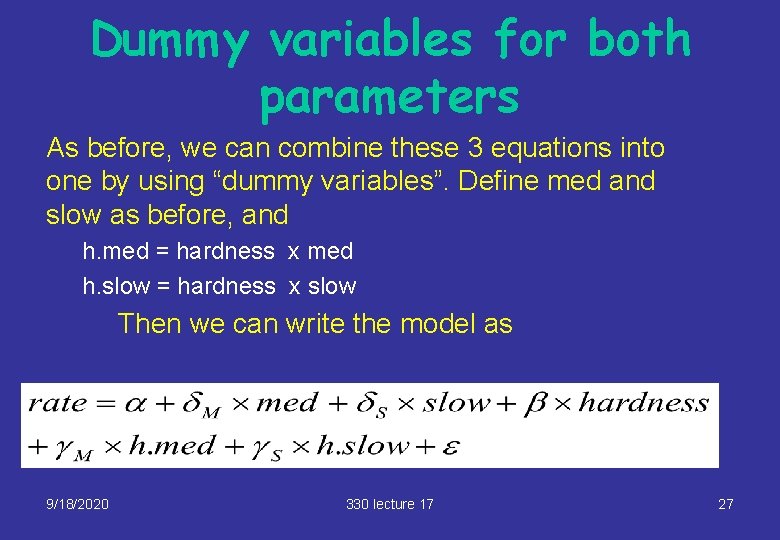
Dummy variables for both parameters As before, we can combine these 3 equations into one by using “dummy variables”. Define med and slow as before, and h. med = hardness x med h. slow = hardness x slow Then we can write the model as 9/18/2020 330 lecture 17 27

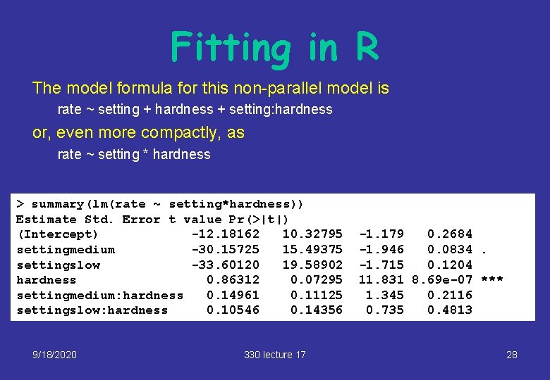
Fitting in R The model formula for this non-parallel model is rate ~ setting + hardness + setting: hardness or, even more compactly, as rate ~ setting * hardness > summary(lm(rate ~ setting*hardness)) Estimate Std. Error t value Pr(>|t|) (Intercept) -12. 18162 10. 32795 settingmedium -30. 15725 15. 49375 settingslow -33. 60120 19. 58902 hardness 0. 86312 0. 07295 settingmedium: hardness 0. 14961 0. 11125 settingslow: hardness 0. 10546 0. 14356 9/18/2020 330 lecture 17 -1. 179 0. 2684 -1. 946 0. 0834. -1. 715 0. 1204 11. 831 8. 69 e-07 *** 1. 345 0. 2116 0. 735 0. 4813 28

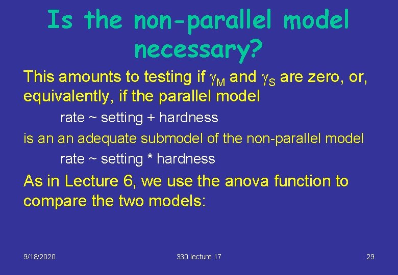
Is the non-parallel model necessary? This amounts to testing if g. M and g. S are zero, or, equivalently, if the parallel model rate ~ setting + hardness is an an adequate submodel of the non-parallel model rate ~ setting * hardness As in Lecture 6, we use the anova function to compare the two models: 9/18/2020 330 lecture 17 29

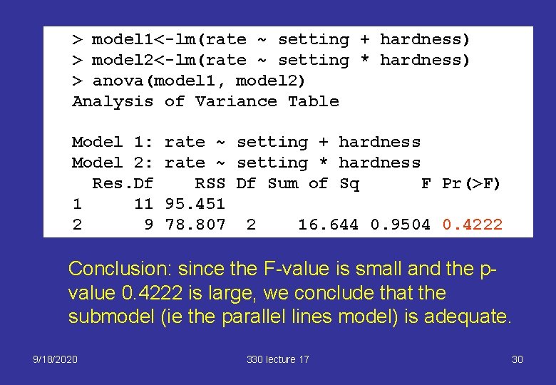
> model 1<-lm(rate ~ setting + hardness) > model 2<-lm(rate ~ setting * hardness) > anova(model 1, model 2) Analysis of Variance Table Model 1: Model 2: Res. Df 1 11 2 9 rate ~ setting + hardness rate ~ setting * hardness RSS Df Sum of Sq F Pr(>F) 95. 451 78. 807 2 16. 644 0. 9504 0. 4222 Conclusion: since the F-value is small and the pvalue 0. 4222 is large, we conclude that the submodel (ie the parallel lines model) is adequate. 9/18/2020 330 lecture 17 30