STATS 330 Lecture 13 1252020 330 lecture 13

STATS 330: Lecture 13 12/5/2020 330 lecture 13 1

Diagnostics 5 Aim of today’s lecture To discuss diagnostics and remedies for non -normality To apply these and the other diagnostics in a case study 12/5/2020 330 lecture 13 2

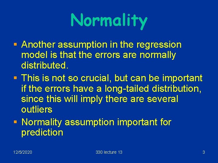
Normality § Another assumption in the regression model is that the errors are normally distributed. § This is not so crucial, but can be important if the errors have a long-tailed distribution, since this will imply there are several outliers § Normality assumption important for prediction 12/5/2020 330 lecture 13 3

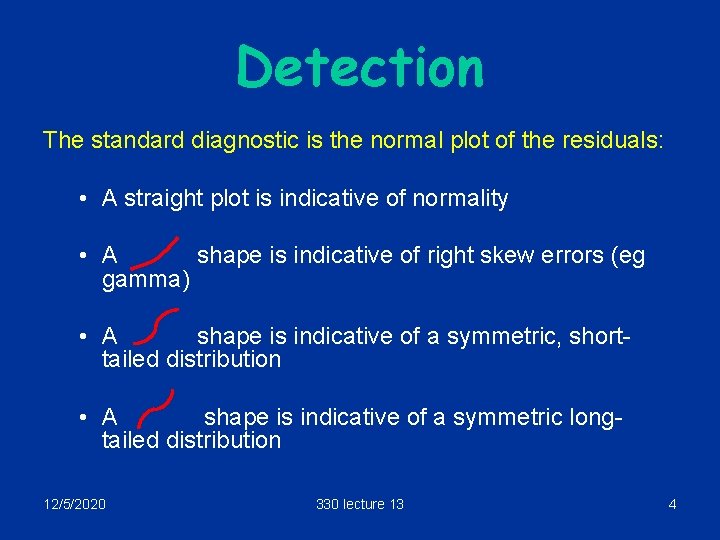
Detection The standard diagnostic is the normal plot of the residuals: • A straight plot is indicative of normality • A shape is indicative of right skew errors (eg gamma) • A shape is indicative of a symmetric, shorttailed distribution • A shape is indicative of a symmetric longtailed distribution 12/5/2020 330 lecture 13 4

qqnorm(residuals(xyz. lm)) Normal errors Right-skew errors Long-tailed errors Short-tailed errors 12/5/2020 330 lecture 13 5

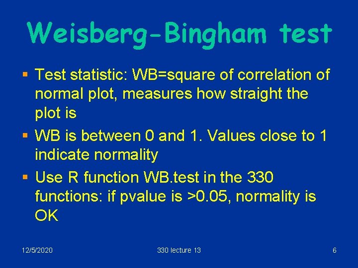
Weisberg-Bingham test § Test statistic: WB=square of correlation of normal plot, measures how straight the plot is § WB is between 0 and 1. Values close to 1 indicate normality § Use R function WB. test in the 330 functions: if pvalue is >0. 05, normality is OK 12/5/2020 330 lecture 13 6

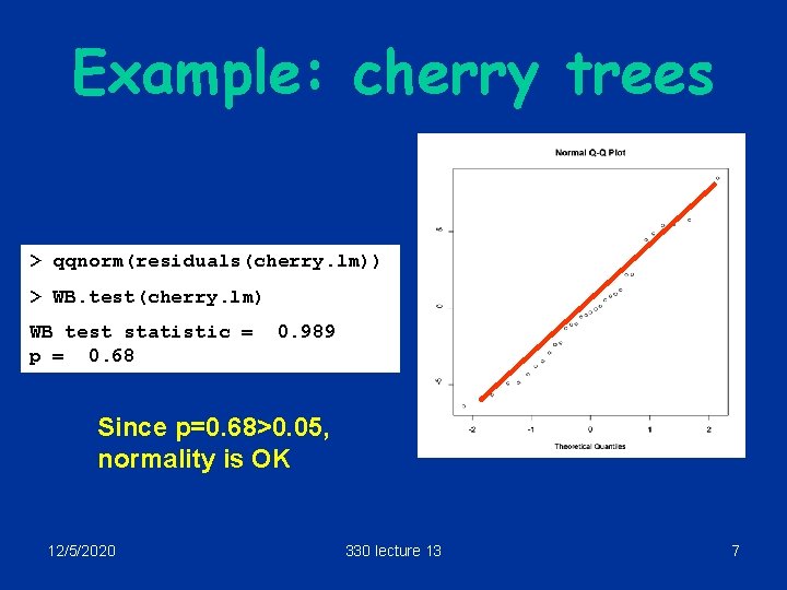
Example: cherry trees > qqnorm(residuals(cherry. lm)) > WB. test(cherry. lm) WB test statistic = p = 0. 68 0. 989 Since p=0. 68>0. 05, normality is OK 12/5/2020 330 lecture 13 7

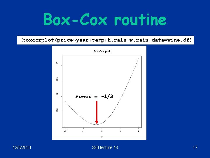
Remedies for non-normality § The standard remedy is to transform the response using a power transformation § The idea is, on the original scale the model doesn’t fit well, but on the transformed scale it does § The power is obtained by means of a “Box-Cox plot” § The idea is to assume that for some power p, the response yp follows the regression model. The plot is a graphical way of estimating the power p. § Technically, it is a plot of the “profile likelihood” 12/5/2020 330 lecture 13 8

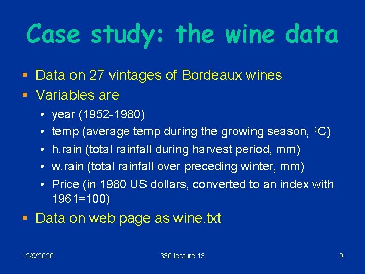
Case study: the wine data § Data on 27 vintages of Bordeaux wines § Variables are • • • year (1952 -1980) temp (average temp during the growing season, o. C) h. rain (total rainfall during harvest period, mm) w. rain (total rainfall over preceding winter, mm) Price (in 1980 US dollars, converted to an index with 1961=100) § Data on web page as wine. txt 12/5/2020 330 lecture 13 9

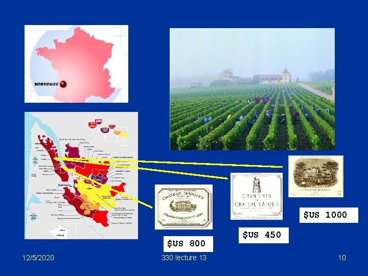
$US 1000 $US 800 12/5/2020 330 lecture 13 $US 450 10

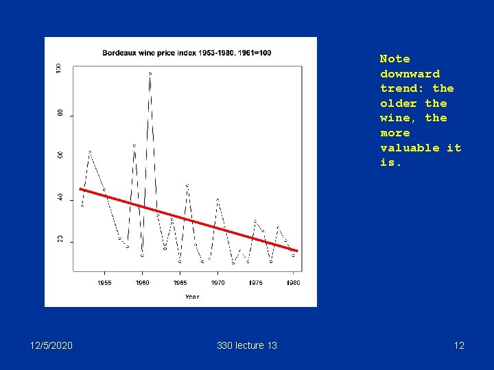
Wine prices § Bordeaux wines are an iconic luxury consumer good. Many consider these to be the best wines in the world. § The quality and the price depends on the vintage (i. e. the year the wines are made. ) § The prices are (in 1980 dollars, in index form, 1961=100) 12/5/2020 330 lecture 13 11

Note downward trend: the older the wine, the more valuable it is. 12/5/2020 330 lecture 13 12

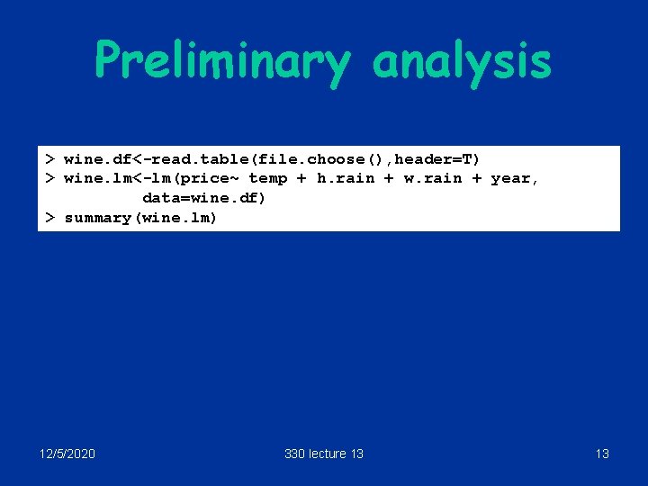
Preliminary analysis > wine. df<-read. table(file. choose(), header=T) > wine. lm<-lm(price~ temp + h. rain + w. rain + year, data=wine. df) > summary(wine. lm) 12/5/2020 330 lecture 13 13

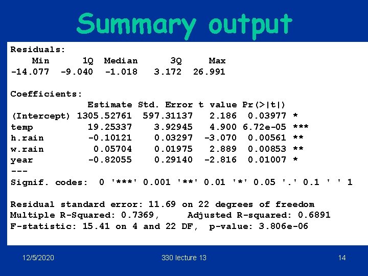
Summary output Residuals: Min 1 Q -14. 077 -9. 040 Median -1. 018 3 Q 3. 172 Max 26. 991 Coefficients: Estimate Std. Error t value Pr(>|t|) (Intercept) 1305. 52761 597. 31137 2. 186 0. 03977 * temp 19. 25337 3. 92945 4. 900 6. 72 e-05 *** h. rain -0. 10121 0. 03297 -3. 070 0. 00561 ** w. rain 0. 05704 0. 01975 2. 889 0. 00853 ** year -0. 82055 0. 29140 -2. 816 0. 01007 * --Signif. codes: 0 '***' 0. 001 '**' 0. 01 '*' 0. 05 '. ' 0. 1 ' ' 1 Residual standard error: 11. 69 on 22 degrees of freedom Multiple R-Squared: 0. 7369, Adjusted R-squared: 0. 6891 F-statistic: 15. 41 on 4 and 22 DF, p-value: 3. 806 e-06 12/5/2020 330 lecture 13 14

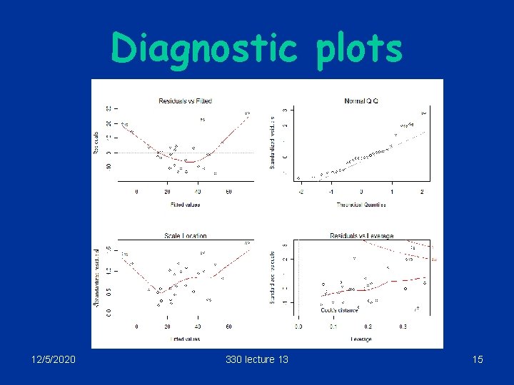
Diagnostic plots 12/5/2020 330 lecture 13 15

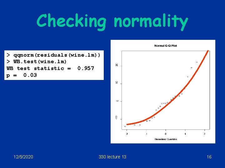
Checking normality > qqnorm(residuals(wine. lm)) > WB. test(wine. lm) WB test statistic = 0. 957 p = 0. 03 12/5/2020 330 lecture 13 16

Box-Cox routine boxcoxplot(price~year+temp+h. rain+w. rain, data=wine. df) Power = -1/3 12/5/2020 330 lecture 13 17

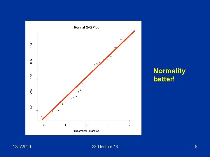
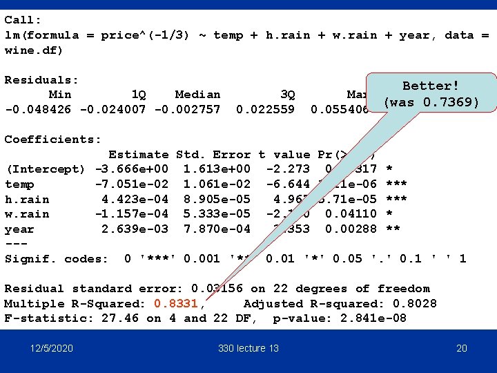
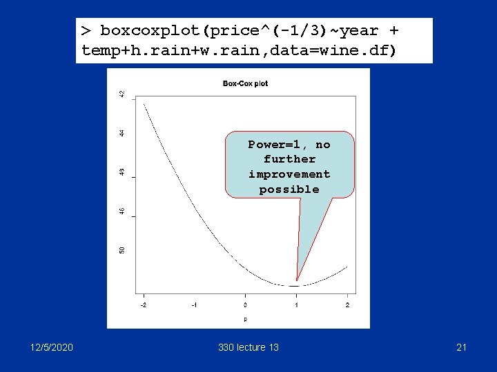
Transform and refit § Use y^(-1/3) as a response (reciprocal cube root) § Has the fit improved? • Are the errors now more normal? (normal plot) • Look at R 2, has R 2 increased? • Could we improve normality by a further transformation? (power=1 means that the fit cannot be improved by further transformation) 12/5/2020 330 lecture 13 18

Normality better! 12/5/2020 330 lecture 13 19

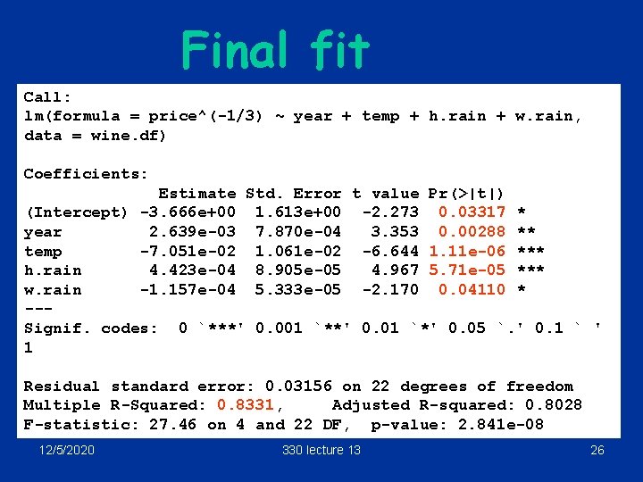
Call: lm(formula = price^(-1/3) ~ temp + h. rain + w. rain + year, data = wine. df) Residuals: Min 1 Q Median -0. 048426 -0. 024007 -0. 002757 3 Q 0. 022559 Better! Max (was 0. 7369) 0. 055406 Coefficients: Estimate Std. Error t value Pr(>|t|) (Intercept) -3. 666 e+00 1. 613 e+00 -2. 273 0. 03317 * temp -7. 051 e-02 1. 061 e-02 -6. 644 1. 11 e-06 *** h. rain 4. 423 e-04 8. 905 e-05 4. 967 5. 71 e-05 *** w. rain -1. 157 e-04 5. 333 e-05 -2. 170 0. 04110 * year 2. 639 e-03 7. 870 e-04 3. 353 0. 00288 ** --Signif. codes: 0 '***' 0. 001 '**' 0. 01 '*' 0. 05 '. ' 0. 1 ' ' 1 Residual standard error: 0. 03156 on 22 degrees of freedom Multiple R-Squared: 0. 8331, Adjusted R-squared: 0. 8028 F-statistic: 27. 46 on 4 and 22 DF, p-value: 2. 841 e-08 12/5/2020 330 lecture 13 20

> boxcoxplot(price^(-1/3)~year + temp+h. rain+w. rain, data=wine. df) Power=1, no further improvement possible 12/5/2020 330 lecture 13 21

Conclusion § Transformation has been spectacularly successful in improving the fit! § What about other aspects of the fit? • residuals/fitted values • Pairs • Partial residual plots 12/5/2020 330 lecture 13 22

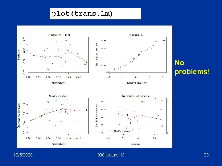
plot(trans. lm) No problems! 12/5/2020 330 lecture 13 23

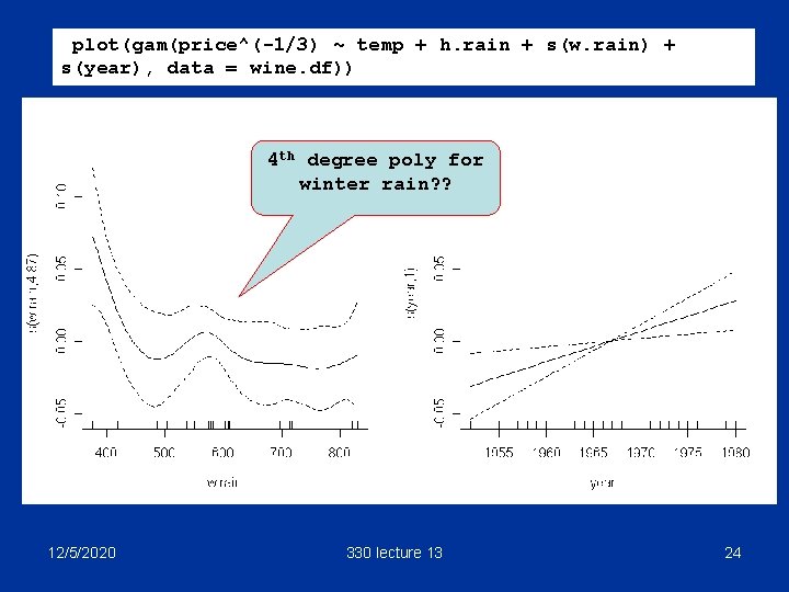
plot(gam(price^(-1/3) ~ temp + h. rain + s(w. rain) + s(year), data = wine. df)) 4 th degree poly for winter rain? ? w. rain better as quadatic? 12/5/2020 330 lecture 13 24

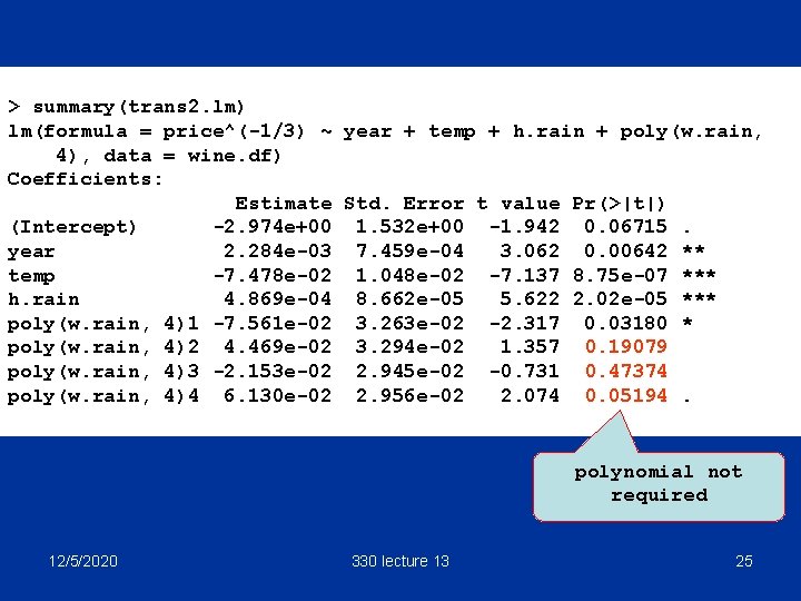
> summary(trans 2. lm) lm(formula = price^(-1/3) ~ year + temp + h. rain + poly(w. rain, 4), data = wine. df) Coefficients: Estimate Std. Error t value Pr(>|t|) (Intercept) -2. 974 e+00 1. 532 e+00 -1. 942 0. 06715. year 2. 284 e-03 7. 459 e-04 3. 062 0. 00642 ** temp -7. 478 e-02 1. 048 e-02 -7. 137 8. 75 e-07 *** h. rain 4. 869 e-04 8. 662 e-05 5. 622 2. 02 e-05 *** poly(w. rain, 4)1 -7. 561 e-02 3. 263 e-02 -2. 317 0. 03180 * poly(w. rain, 4)2 4. 469 e-02 3. 294 e-02 1. 357 0. 19079 poly(w. rain, 4)3 -2. 153 e-02 2. 945 e-02 -0. 731 0. 47374 poly(w. rain, 4)4 6. 130 e-02 2. 956 e-02 2. 074 0. 05194. polynomial not required 12/5/2020 330 lecture 13 25

Final fit Call: lm(formula = price^(-1/3) ~ year + temp + h. rain + w. rain, data = wine. df) Coefficients: Estimate Std. Error t value Pr(>|t|) (Intercept) -3. 666 e+00 1. 613 e+00 -2. 273 0. 03317 * year 2. 639 e-03 7. 870 e-04 3. 353 0. 00288 ** temp -7. 051 e-02 1. 061 e-02 -6. 644 1. 11 e-06 *** h. rain 4. 423 e-04 8. 905 e-05 4. 967 5. 71 e-05 *** w. rain -1. 157 e-04 5. 333 e-05 -2. 170 0. 04110 * --Signif. codes: 0 `***' 0. 001 `**' 0. 01 `*' 0. 05 `. ' 0. 1 ` ' 1 Residual standard error: 0. 03156 on 22 degrees of freedom Multiple R-Squared: 0. 8331, Adjusted R-squared: 0. 8028 F-statistic: 27. 46 on 4 and 22 DF, p-value: 2. 841 e-08 12/5/2020 330 lecture 13 26

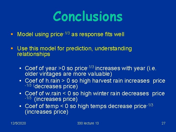
Conclusions § Model using price-1/3 as response fits well § Use this model for prediction, understanding relationships • Coef of year >0 so price-1/3 increases with year (i. e. older vintages are more valuable) • Coef of h. rain > 0 so high harvest rain increases price -1/3 (decreases price) • Coef of w. rain < 0 so high winter rain decreases price -1/3 (increases price) • Coef of temp < 0 so high temps decrease price-1/3 (increases price) 12/5/2020 330 lecture 13 27

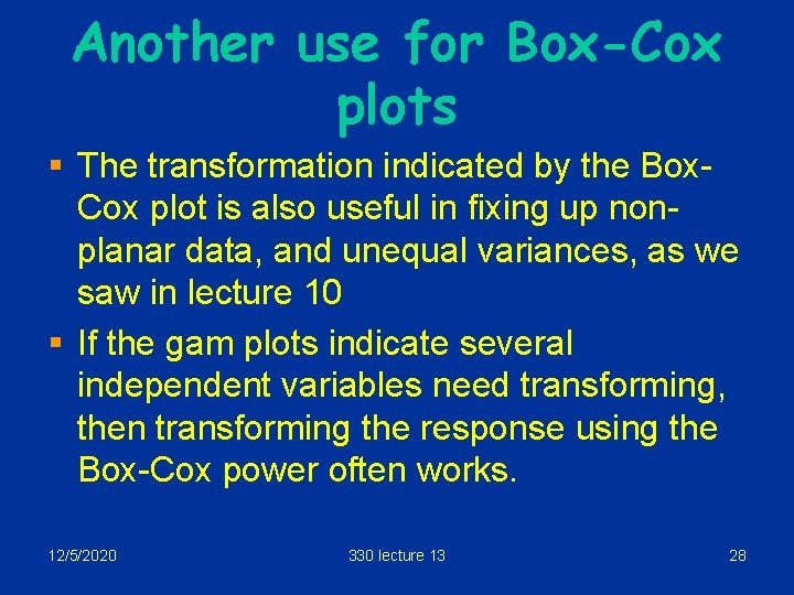
Another use for Box-Cox plots § The transformation indicated by the Box. Cox plot is also useful in fixing up nonplanar data, and unequal variances, as we saw in lecture 10 § If the gam plots indicate several independent variables need transforming, then transforming the response using the Box-Cox power often works. 12/5/2020 330 lecture 13 28