STATS 330 Lecture 3 9252020 330 lecture 3

STATS 330: Lecture 3 9/25/2020 330 lecture 3 1

Class Rep ? ? ? ? ? 9/25/2020 330 lecture 3 2

Today’s lecture: More on Trellis graphics Aim of the lecture: § To give you an idea of the scope of trellis graphics § To discuss several examples and show Trellis graphics reveal important insights into the data 9/25/2020 330 lecture 3 3

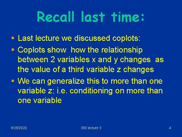
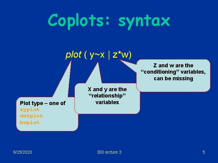
Recall last time: § Last lecture we discussed coplots: § Coplots show the relationship between 2 variables x and y changes as the value of a third variable z changes § We can generalize this to more than one variable z: i. e. conditioning on more than one variable 9/25/2020 330 lecture 3 4

Coplots: syntax plot ( y~x | z*w) Z and w are the “conditioning” variables, can be missing Plot type – one of xyplot dotplot bwplot 9/25/2020 X and y are the “relationship” variables 330 lecture 3 5

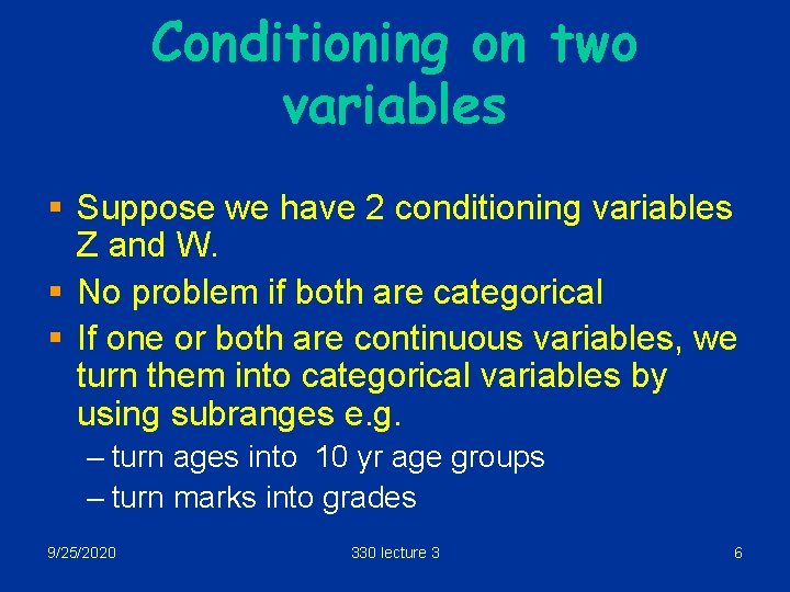
Conditioning on two variables § Suppose we have 2 conditioning variables Z and W. § No problem if both are categorical § If one or both are continuous variables, we turn them into categorical variables by using subranges e. g. – turn ages into 10 yr age groups – turn marks into grades 9/25/2020 330 lecture 3 6

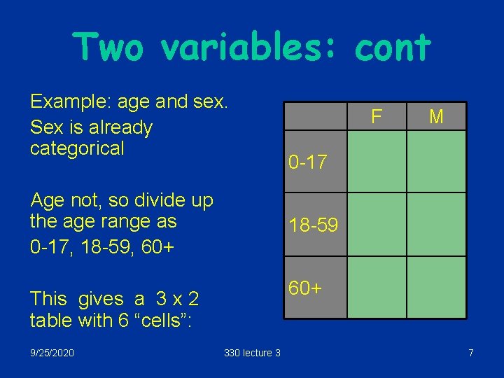
Two variables: cont Example: age and sex. Sex is already categorical Age not, so divide up the age range as 0 -17, 18 -59, 60+ M 0 -17 18 -59 60+ This gives a 3 x 2 table with 6 “cells”: 9/25/2020 F 330 lecture 3 7

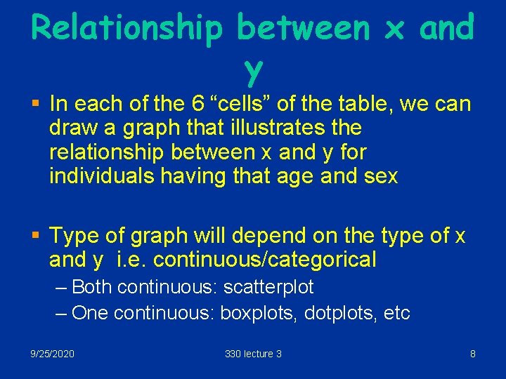
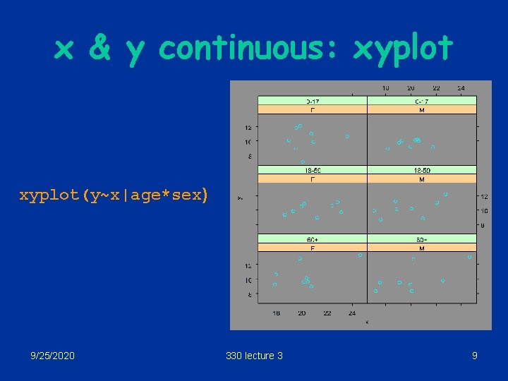
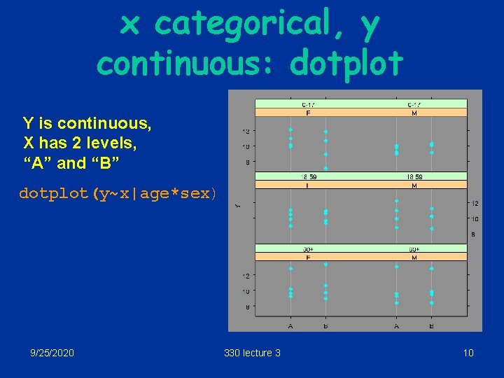
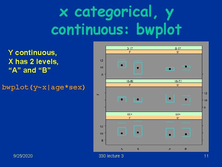
Relationship between x and y § In each of the 6 “cells” of the table, we can draw a graph that illustrates the relationship between x and y for individuals having that age and sex § Type of graph will depend on the type of x and y i. e. continuous/categorical – Both continuous: scatterplot – One continuous: boxplots, dotplots, etc 9/25/2020 330 lecture 3 8

x & y continuous: xyplot(y~x|age*sex) 9/25/2020 330 lecture 3 9

x categorical, y continuous: dotplot Y is continuous, X has 2 levels, “A” and “B” dotplot(y~x|age*sex) 9/25/2020 330 lecture 3 10

x categorical, y continuous: bwplot Y continuous, X has 2 levels, “A” and “B” bwplot(y~x|age*sex) 9/25/2020 330 lecture 3 11

To summarize: § The conditioning variables determine the layout of the “cells” § The x/y variables determine the kind of graph to draw in each cell 9/25/2020 330 lecture 3 12

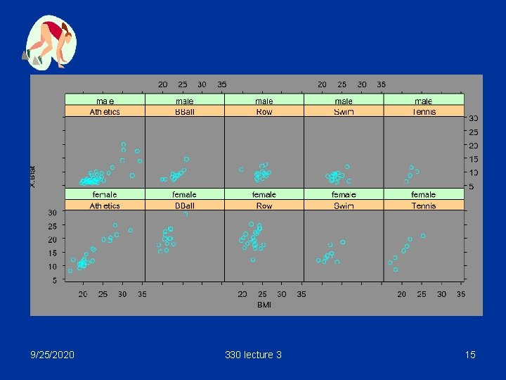
Example: sports § In a study on athletes at the Australian Institute of Sport, various physical measurements were made. § In this example we look at the relationship between body fat and BMI and how it differs between athletes of either sex playing different sports. BMI = weight(kg) / height(m)2 9/25/2020 330 lecture 3 13

Data 1 2 3 4 5 6 7 8 9 10 sex female female female sport BBall BBall BBall BMI X. Bfat 20. 56 19. 75 20. 67 21. 30 21. 86 19. 88 21. 88 23. 66 18. 96 17. 64 21. 04 15. 58 21. 69 19. 99 20. 62 22. 43 22. 64 17. 95 19. 44 15. 07 … more data (158 lines in all) 9/25/2020 330 lecture 3 14

9/25/2020 330 lecture 3 15

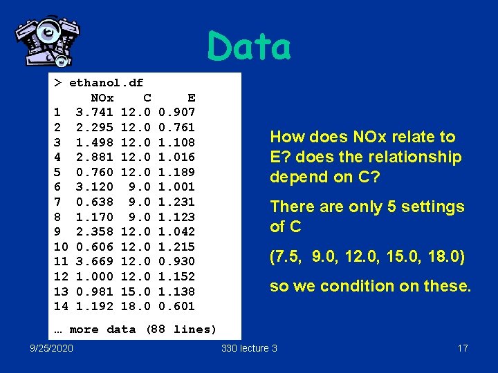
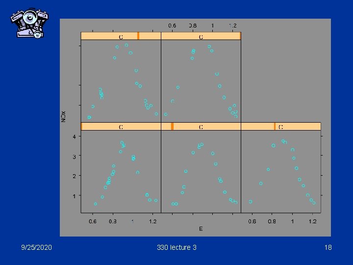
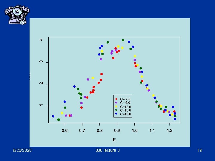
Example: engines § In a study of engine emissions, a test engine was run under different conditions and the amount of nitrogen oxide (NOx) emitted was measured. § The conditions involved different settings of the compression ratio C, and the Equivalence ratio, E (related to fuel/air mixture) 9/25/2020 330 lecture 3 16

Data > ethanol. df NOx C 1 3. 741 12. 0 2 2. 295 12. 0 3 1. 498 12. 0 4 2. 881 12. 0 5 0. 760 12. 0 6 3. 120 9. 0 7 0. 638 9. 0 8 1. 170 9. 0 9 2. 358 12. 0 10 0. 606 12. 0 11 3. 669 12. 0 12 1. 000 12. 0 13 0. 981 15. 0 14 1. 192 18. 0 E 0. 907 0. 761 1. 108 1. 016 1. 189 1. 001 1. 231 1. 123 1. 042 1. 215 0. 930 1. 152 1. 138 0. 601 How does NOx relate to E? does the relationship depend on C? There are only 5 settings of C (7. 5, 9. 0, 12. 0, 15. 0, 18. 0) so we condition on these. … more data (88 lines) 9/25/2020 330 lecture 3 17

9/25/2020 330 lecture 3 18

9/25/2020 330 lecture 3 19

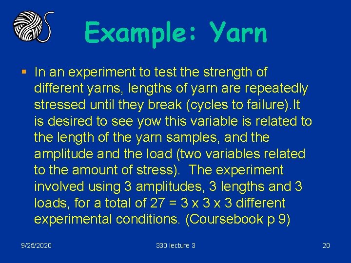
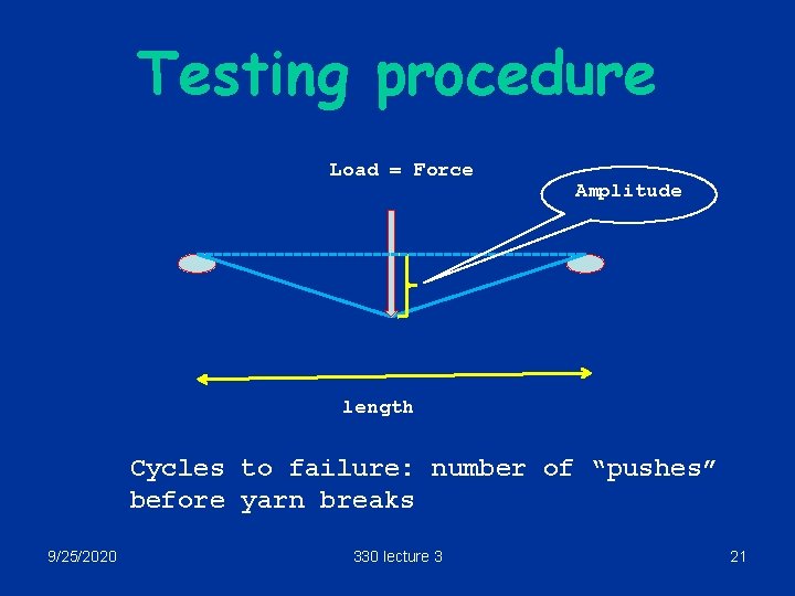
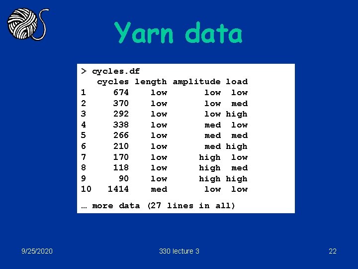
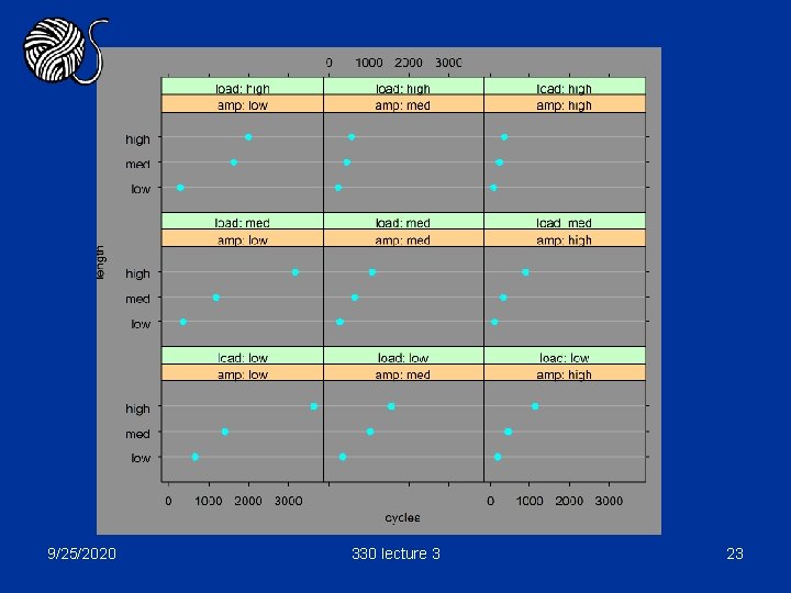
Example: Yarn § In an experiment to test the strength of different yarns, lengths of yarn are repeatedly stressed until they break (cycles to failure). It is desired to see yow this variable is related to the length of the yarn samples, and the amplitude and the load (two variables related to the amount of stress). The experiment involved using 3 amplitudes, 3 lengths and 3 loads, for a total of 27 = 3 x 3 different experimental conditions. (Coursebook p 9) 9/25/2020 330 lecture 3 20

Testing procedure Load = Force Amplitude length Cycles to failure: number of “pushes” before yarn breaks 9/25/2020 330 lecture 3 21

Yarn data > cycles. df cycles length amplitude load 1 674 low low 2 370 low med 3 292 low high 4 338 low med low 5 266 low med 6 210 low med high 7 170 low high low 8 118 low high med 9 90 low high 10 1414 med low … more data (27 lines in all) 9/25/2020 330 lecture 3 22

9/25/2020 330 lecture 3 23

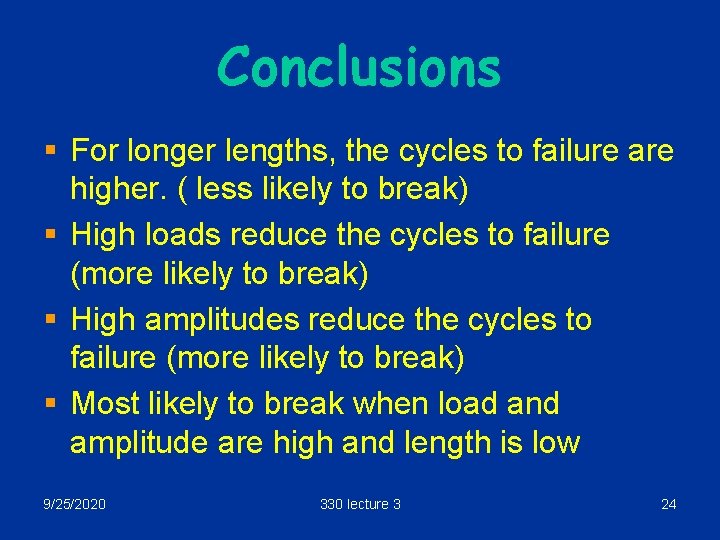
Conclusions § For longer lengths, the cycles to failure are higher. ( less likely to break) § High loads reduce the cycles to failure (more likely to break) § High amplitudes reduce the cycles to failure (more likely to break) § Most likely to break when load and amplitude are high and length is low 9/25/2020 330 lecture 3 24