STATS 330 Lecture 11 1122022 330 lecture 11

STATS 330: Lecture 11 1/12/2022 330 lecture 11 1

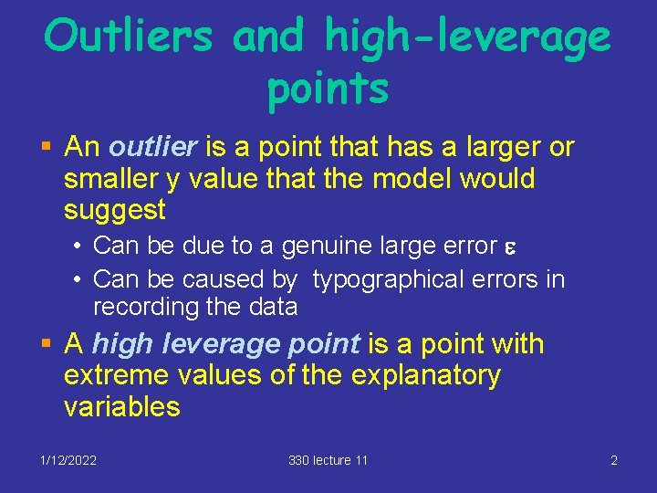
Outliers and high-leverage points § An outlier is a point that has a larger or smaller y value that the model would suggest • Can be due to a genuine large error e • Can be caused by typographical errors in recording the data § A high leverage point is a point with extreme values of the explanatory variables 1/12/2022 330 lecture 11 2

Outliers § The effect of an outlier depends on whether it is also a high leverage point § A “high leverage” outlier • Can attract the fitted plane, distorting the fit, sometimes extremely • In extreme cases may not have a big residual • In extreme cases can increase R 2 § A “low leverage” outlier • Does not distort the fit to the same extent • Usually has a big residual • Inflates standard errors, decreases R 2 1/12/2022 330 lecture 11 3

No outliers No highleverage points Low leverage Outlier: big residual High leverage Not an outlier 1/12/2022 Highleverage outlier 330 lecture 11 4

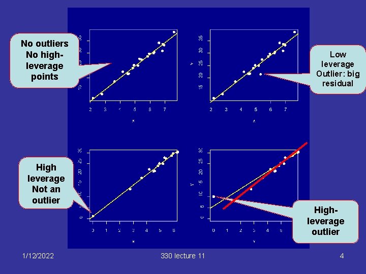
Example: the education data (ignoring urban) High leverage point 1/12/2022 330 lecture 11 5

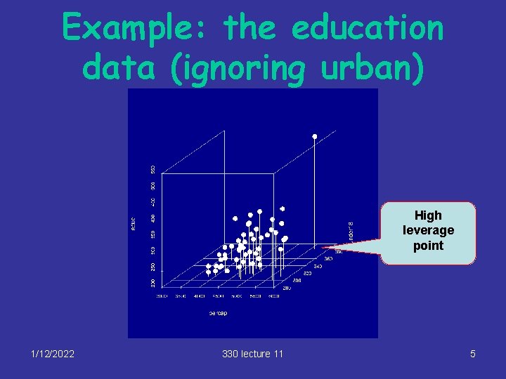
An outlier also? Residual somewhat extreme 1/12/2022 330 lecture 11 6

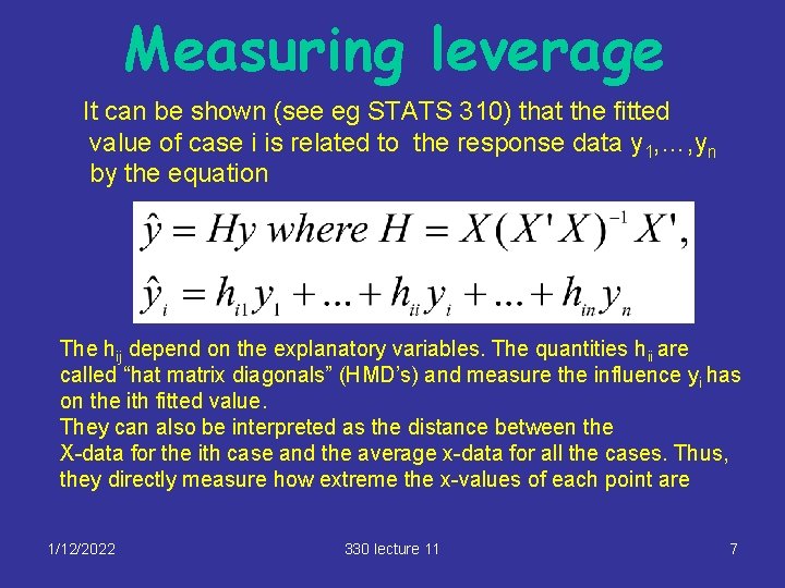
Measuring leverage It can be shown (see eg STATS 310) that the fitted value of case i is related to the response data y 1, …, yn by the equation The hij depend on the explanatory variables. The quantities hii are called “hat matrix diagonals” (HMD’s) and measure the influence yi has on the ith fitted value. They can also be interpreted as the distance between the X-data for the ith case and the average x-data for all the cases. Thus, they directly measure how extreme the x-values of each point are 1/12/2022 330 lecture 11 7

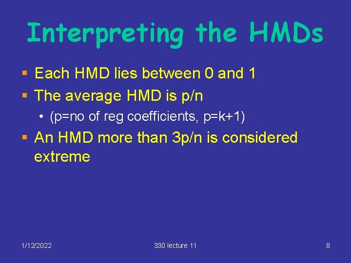
Interpreting the HMDs § Each HMD lies between 0 and 1 § The average HMD is p/n • (p=no of reg coefficients, p=k+1) § An HMD more than 3 p/n is considered extreme 1/12/2022 330 lecture 11 8

Example: the education data educ. lm<-lm(educ~percapita+under 18, data=educ. df) hatvalues(educ. lm)[50] 50 0. 3428523 n=50, p=3 > 9/50 [1] 0. 18 Clearly extreme! 1/12/2022 330 lecture 11 9

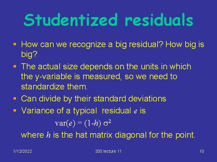
Studentized residuals § How can we recognize a big residual? How big is big? § The actual size depends on the units in which the y-variable is measured, so we need to standardize them. § Can divide by their standard deviations § Variance of a typical residual e is var(e) = (1 -h) s 2 where h is the hat matrix diagonal for the point. 1/12/2022 330 lecture 11 10

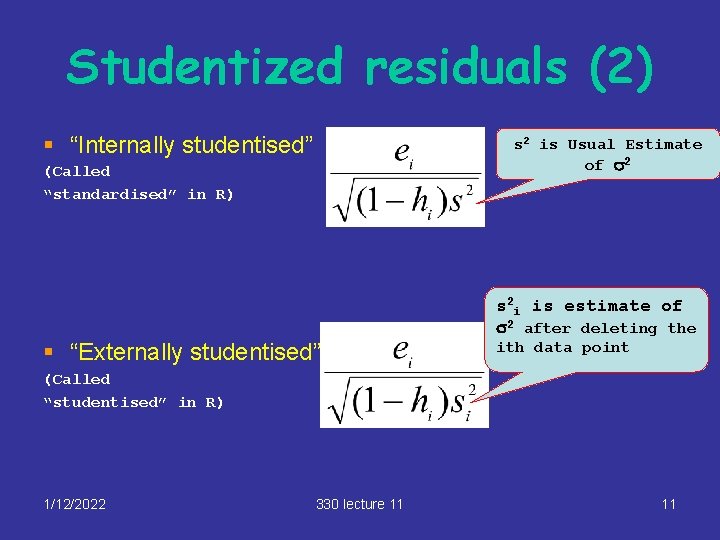
Studentized residuals (2) § “Internally studentised” s 2 is Usual Estimate of s 2 (Called “standardised” in R) s 2 i is estimate of s 2 after deleting the § “Externally studentised” ith data point (Called “studentised” in R) 1/12/2022 330 lecture 11 11

Studentized residuals (3) § How big is big? § Both types of studentised residual are approximately distributed as standard normals when the model is OK and there are no outliers. (in fact the externally studentised one has a tdistribution) § Thus, studentised residuals should be between 2 and 2 with approximately 95% probability. 1/12/2022 330 lecture 11 12

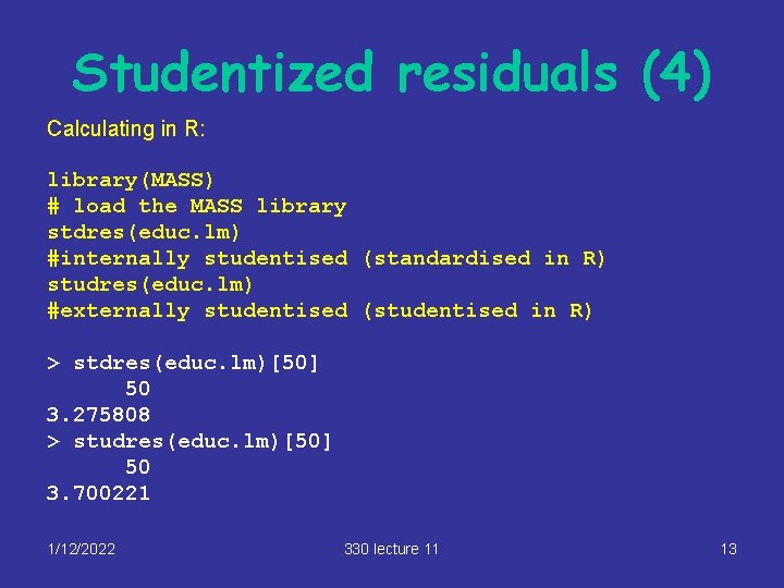
Studentized residuals (4) Calculating in R: library(MASS) # load the MASS library stdres(educ. lm) #internally studentised (standardised in R) studres(educ. lm) #externally studentised (studentised in R) > stdres(educ. lm)[50] 50 3. 275808 > studres(educ. lm)[50] 50 3. 700221 1/12/2022 330 lecture 11 13

What does studentised mean? 1/12/2022 330 lecture 11 14

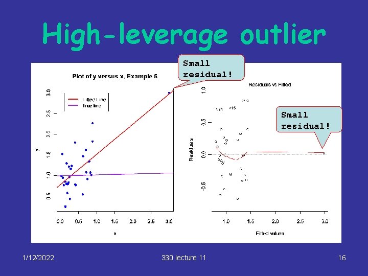
Recognizing outliers § If a point is a low influence outlier, the residual will usually be large, so large residual and a low HMD indicates an outlier § If a point is a high leverage outlier, then a large error usually will cause a large residual. § However, in extreme cases, a high leverage outlier may not have a very big residual, depending on how much the point attracts the fitted plane. Thus, if a point has a large HMD, and the residual is not particularly big, we can’t always tell if a point is an outlier or not. 1/12/2022 330 lecture 11 15

High-leverage outlier Small residual! 1/12/2022 330 lecture 11 16

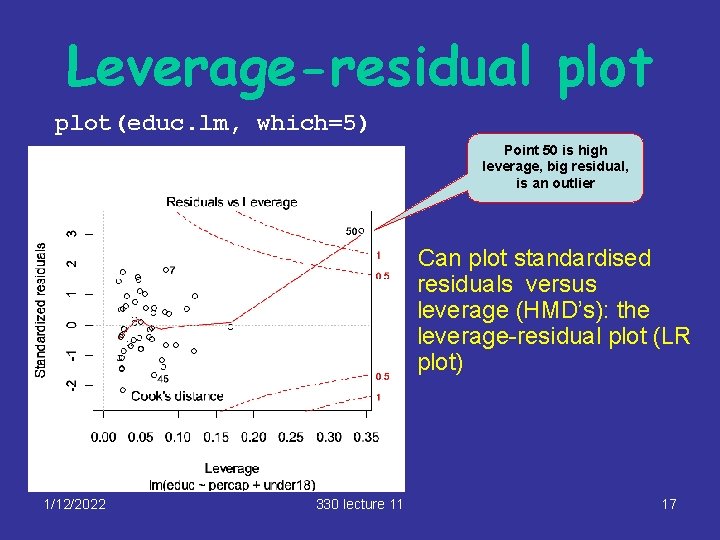
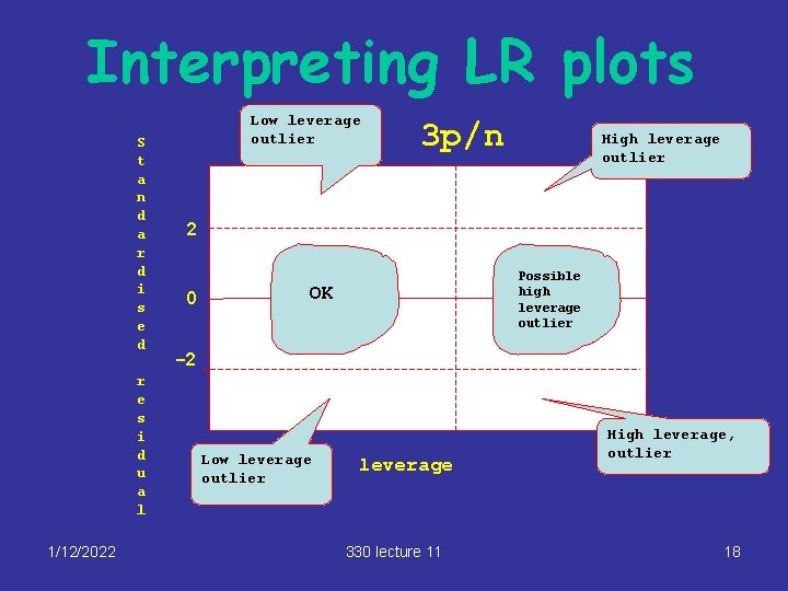
Leverage-residual plot(educ. lm, which=5) Point 50 is high leverage, big residual, is an outlier Can plot standardised residuals versus leverage (HMD’s): the leverage-residual plot (LR plot) 1/12/2022 330 lecture 11 17

Interpreting LR plots S t a n d a r d i s e d r e s i d u a l 1/12/2022 Low leverage outlier 3 p/n High leverage outlier 2 0 Possible high leverage outlier OK -2 Low leverage outlier leverage 330 lecture 11 High leverage, outlier 18

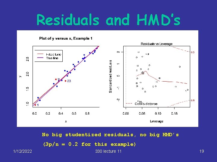
Residuals and HMD’s No big studentized residuals, no big HMD’s (3 p/n = 0. 2 for this example) 1/12/2022 330 lecture 11 19

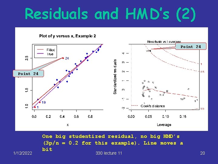
Residuals and HMD’s (2) Point 24 1/12/2022 One big studentized residual, no big HMD’s (3 p/n = 0. 2 for this example). Line moves a bit 330 lecture 11 20

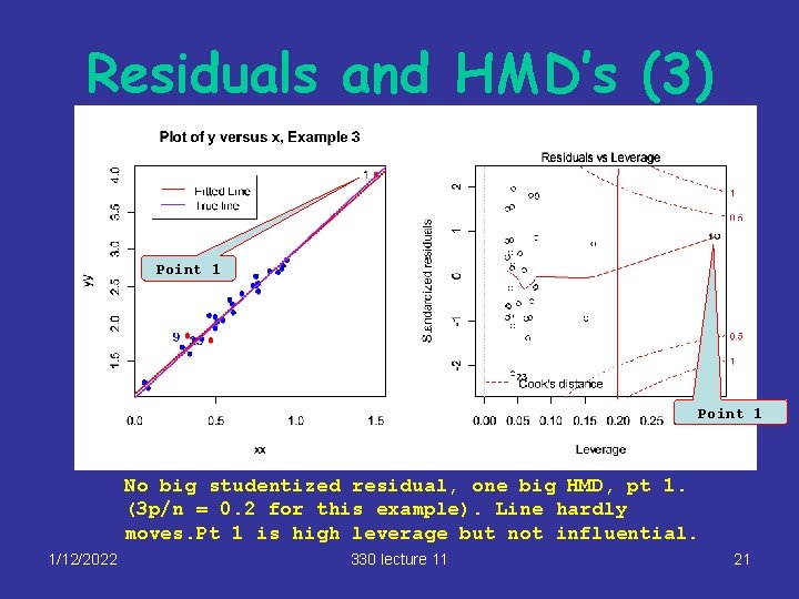
Residuals and HMD’s (3) Point 1 No big studentized residual, one big HMD, pt 1. (3 p/n = 0. 2 for this example). Line hardly moves. Pt 1 is high leverage but not influential. 1/12/2022 330 lecture 11 21

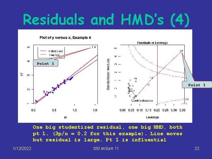
Residuals and HMD’s (4) Point 1 One big studentized residual, one big HMD, both pt 1. (3 p/n = 0. 2 for this example). Line moves but residual is large. Pt 1 is influential 1/12/2022 330 lecture 11 22

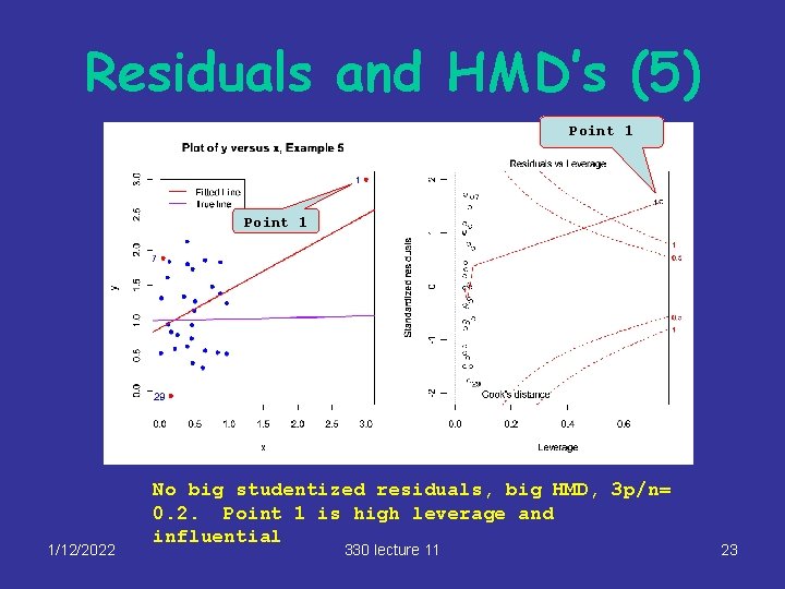
Residuals and HMD’s (5) Point 1 1/12/2022 No big studentized residuals, big HMD, 3 p/n= 0. 2. Point 1 is high leverage and influential 330 lecture 11 23

Influential points § How can we tell if a high-leverage point/outlier is affecting the regression? § By deleting the point and refitting the regression: a large change in coefficients means the point is affecting the regression § Such points are called influential points § Don’t want analysis to be driven by one or two points 1/12/2022 330 lecture 11 24

“Leave-one out” measures § We can calculate a variety of measures by leaving out each data point in turn, and looking at the change in key regression quantities such as • Coefficients • Fitted values • Standard errors § We discuss each in turn 1/12/2022 330 lecture 11 25

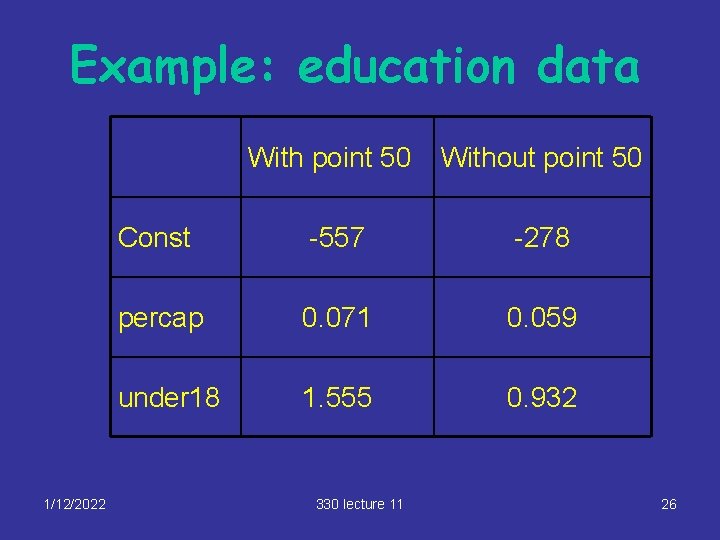
Example: education data 1/12/2022 With point 50 Without point 50 Const -557 -278 percap 0. 071 0. 059 under 18 1. 555 0. 932 330 lecture 11 26

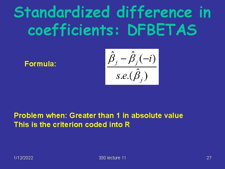
Standardized difference in coefficients: DFBETAS Formula: Problem when: Greater than 1 in absolute value This is the criterion coded into R 1/12/2022 330 lecture 11 27

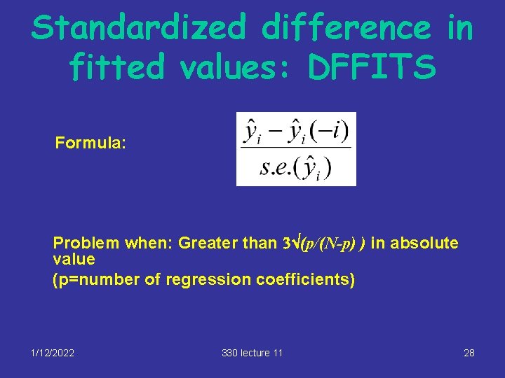
Standardized difference in fitted values: DFFITS Formula: Problem when: Greater than 3Ö(p/(N-p) ) in absolute value (p=number of regression coefficients) 1/12/2022 330 lecture 11 28

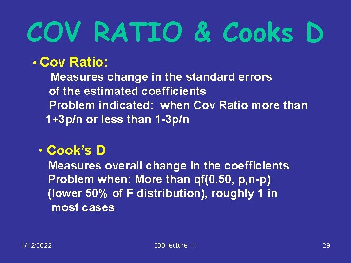
COV RATIO & Cooks D • Cov Ratio: Measures change in the standard errors of the estimated coefficients Problem indicated: when Cov Ratio more than 1+3 p/n or less than 1 -3 p/n • Cook’s D Measures overall change in the coefficients Problem when: More than qf(0. 50, p, n-p) (lower 50% of F distribution), roughly 1 in most cases 1/12/2022 330 lecture 11 29

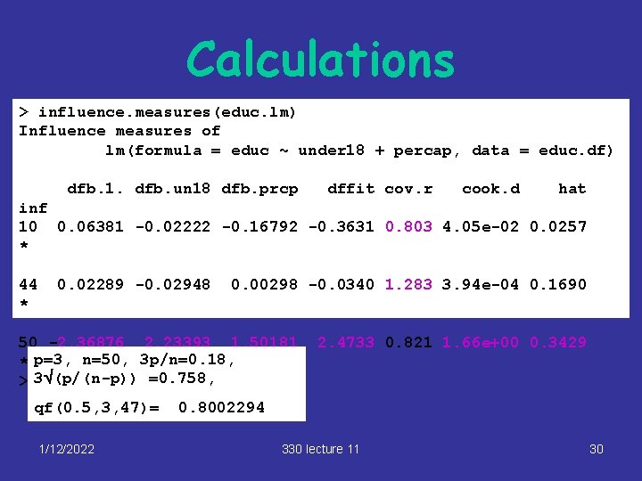
Calculations > influence. measures(educ. lm) Influence measures of lm(formula = educ ~ under 18 + percap, data = educ. df) dfb. 1. dfb. un 18 dfb. prcp dffit cov. r cook. d hat inf 10 0. 06381 -0. 02222 -0. 16792 -0. 3631 0. 803 4. 05 e-02 0. 0257 * 44 * 0. 02289 -0. 02948 0. 00298 -0. 0340 1. 283 3. 94 e-04 0. 1690 50 -2. 36876 2. 23393 1. 50181 * p=3, n=50, 3 p/n=0. 18, > 3Ö(p/(n-p)) =0. 758, qf(0. 5, 3, 47)= 1/12/2022 2. 4733 0. 821 1. 66 e+00 0. 3429 0. 8002294 330 lecture 11 30

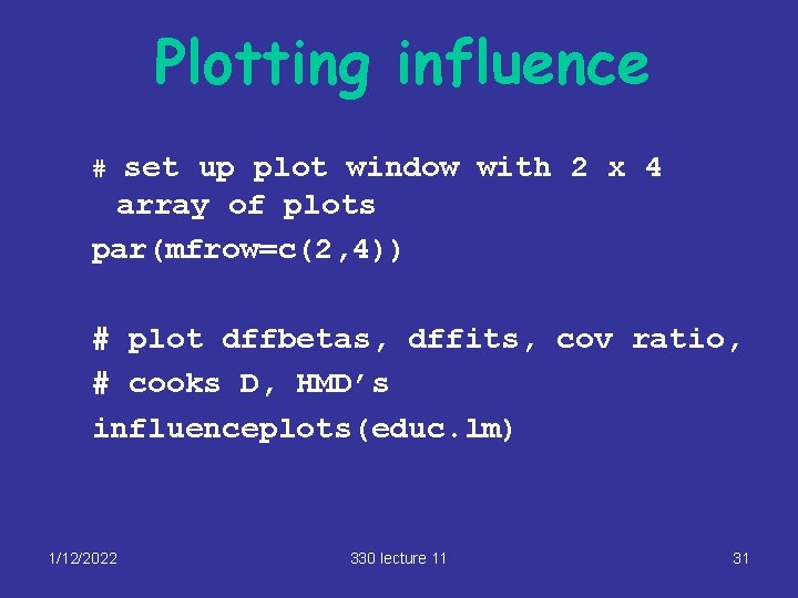
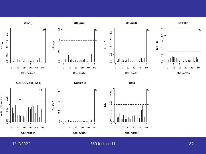
Plotting influence # set up plot window with 2 x 4 array of plots par(mfrow=c(2, 4)) # plot dffbetas, dffits, cov ratio, # cooks D, HMD’s influenceplots(educ. lm) 1/12/2022 330 lecture 11 31

1/12/2022 330 lecture 11 32

Remedies for outliers § Correct typographical errors in the data § Delete a small number of points and refit (don’t want fitted regression to be determined by one or two influential points) § Report existence of outliers separately: they are often of scientific interest § Don’t delete too many points (1 or 2 max) 1/12/2022 330 lecture 11 33

Summary: Doing it in R § LR plot: plot(educ. lm, which=5) § Full diagnostic display plot(educ. lm) § Influence measures: influence. measures(educ. lm) § Plots of influence measures par(mfrow=c(2, 4)) influenceplots(educ. lm) 1/12/2022 330 lecture 11 34

HMD Summary § Hat matrix diagonals • Measure the effect of a point on its fitted value • Measure how outlying the x-values are (how “high –leverage” a point is) • Are always between 0 and 1 with bigger values indicating high leverage • Points with HMD’s more than 3 p/n are considered “high leverage” 1/12/2022 330 lecture 11 35