STATS 330 Lecture 2 10302020 330 Lecture 2

STATS 330: Lecture 2 10/30/2020 330 Lecture 2 1

Housekeeping matters • STATS 762 – An extra test (details to be provided). An extra assignment • Class rep – ? ? • Office hours – Alan: 10: 30 – 12: 00 Tuesday and Thursday in Rm 265, Building 303 S – Tutors: TBA • Assignment 1: Due 2 August 10/30/2020 330 Lecture 2 2

Today’s lecture: Exploratory graphics Aim of the lecture: To give you a quick overview of the kinds of graphs that can be helpful in exploring data. Some of this material has been covered in 201/8. (We will discuss the R code used to make the plots in Lecture 4) 10/30/2020 330 Lecture 2 3

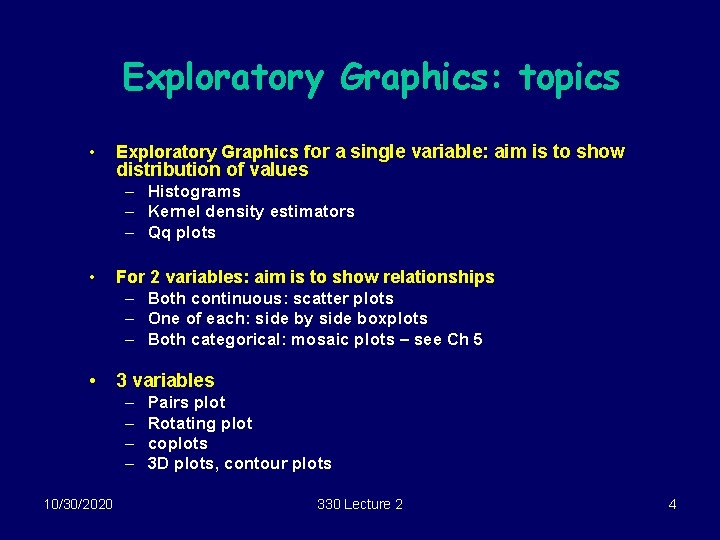
Exploratory Graphics: topics • Exploratory Graphics for a single variable: aim is to show distribution of values – Histograms – Kernel density estimators – Qq plots • For 2 variables: aim is to show relationships – Both continuous: scatter plots – One of each: side by side boxplots – Both categorical: mosaic plots – see Ch 5 • 3 variables – – 10/30/2020 Pairs plot Rotating plot coplots 3 D plots, contour plots 330 Lecture 2 4

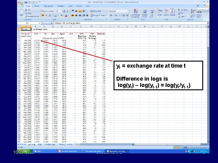
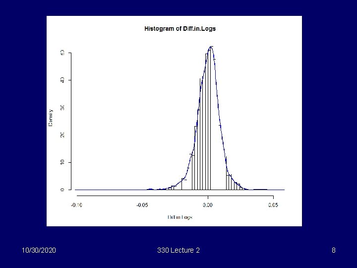
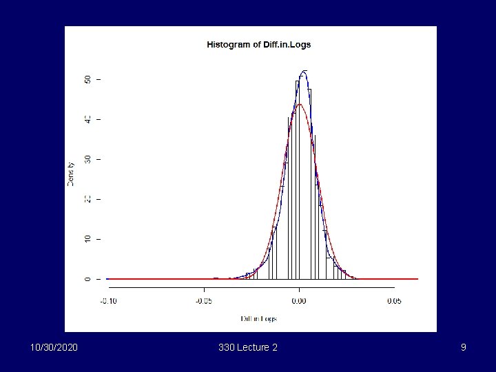
Single variable: Exchange rate data • The data of interest: daily changes in log(exchange rate) for the US$/Kiwi. – Monthly date from June 1986 to may 2012 – Source: Reserve Bank • Questions: – What is the distribution of the daily changes in the logged exchange rate? – Is it normal? If not, how is it different? 10/30/2020 330 Lecture 2 5

yt = exchange rate at time t Difference in logs is log(yt) – log(yt-1) = log(yt/yt-1) 10/30/2020 330 Lecture 2 6

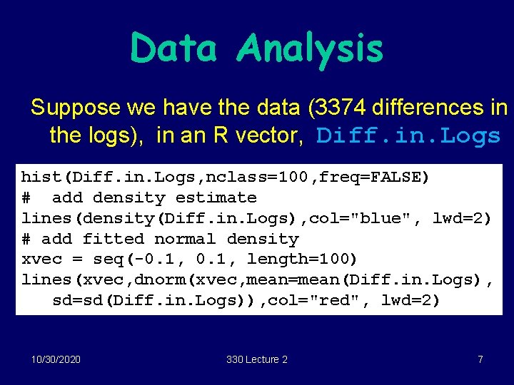
Data Analysis Suppose we have the data (3374 differences in the logs), in an R vector, Diff. in. Logs hist(Diff. in. Logs, nclass=100, freq=FALSE) # add density estimate lines(density(Diff. in. Logs), col="blue", lwd=2) # add fitted normal density xvec = seq(-0. 1, length=100) lines(xvec, dnorm(xvec, mean=mean(Diff. in. Logs), sd=sd(Diff. in. Logs)), col="red", lwd=2) 10/30/2020 330 Lecture 2 7

10/30/2020 330 Lecture 2 8

10/30/2020 330 Lecture 2 9

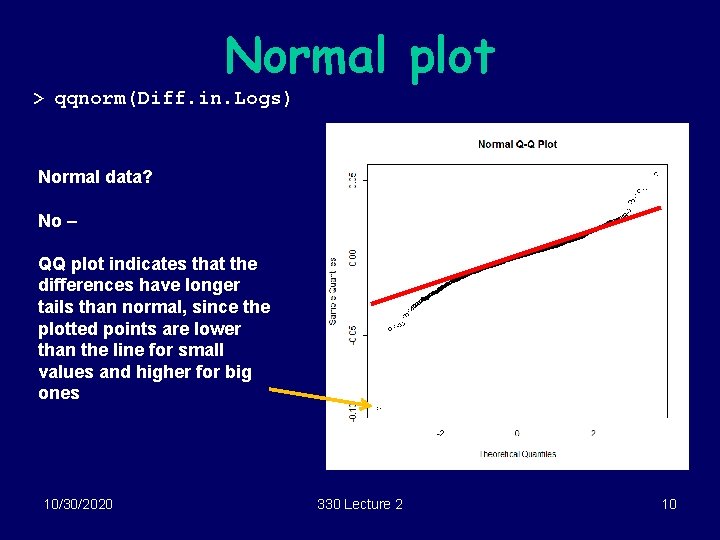
Normal plot > qqnorm(Diff. in. Logs) Normal data? No – QQ plot indicates that the differences have longer tails than normal, since the plotted points are lower than the line for small values and higher for big ones 10/30/2020 330 Lecture 2 10

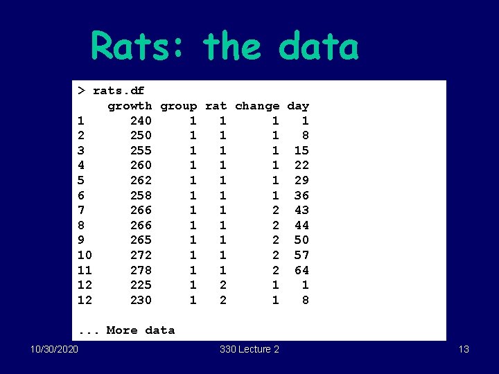
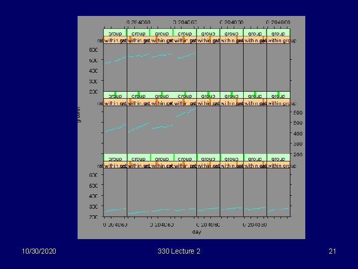
Two Variables: Rats! Of interest: growth rates of 16 rats i. e. relationship between weight and time • Want to explore the relationship graphically. • Each rat was measured (roughly) every week for 11 weeks • For weeks 1 -6, all rats were on a fixed diet. Diet was changed after week 6. 10/30/2020 330 Lecture 2 11

Two Variables: Rats! Data set rats. df has variables – rat (1 -16) – growth (weight in grams) – day (day since start of study, 11 values, at approximately weekly intervals – group (litter, one of 3) – change (has values 1 or 2 - diet was changed after 6 weeks, diet 1 for weeks 1 -6, diet 2 for weeks 7 -11 10/30/2020 330 Lecture 2 12

Rats: the data > rats. df growth group rat change day 1 240 1 1 2 250 1 1 1 8 3 255 1 15 4 260 1 1 1 22 5 262 1 1 1 29 6 258 1 1 1 36 7 266 1 1 2 43 8 266 1 1 2 44 9 265 1 1 2 50 10 272 1 1 2 57 11 278 1 1 2 64 12 225 1 2 1 1 12 230 1 2 1 8. . . More data 10/30/2020 330 Lecture 2 13

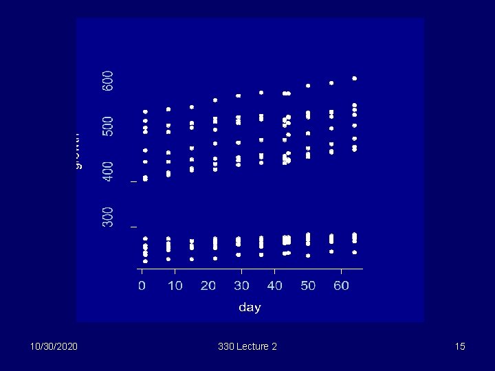
Rats (cont) • Could plot weight (i. e. the variable growth) versus the variable day: plot(day, growth) BUT…. 10/30/2020 330 Lecture 2 14

10/30/2020 330 Lecture 2 15

Criticisms • Can’t tell which points belong to which rat • Seem to be 2 groups of points • In actual fact, the rats came from 3 different litters, is this relevant? • Could do better 10/30/2020 330 Lecture 2 16

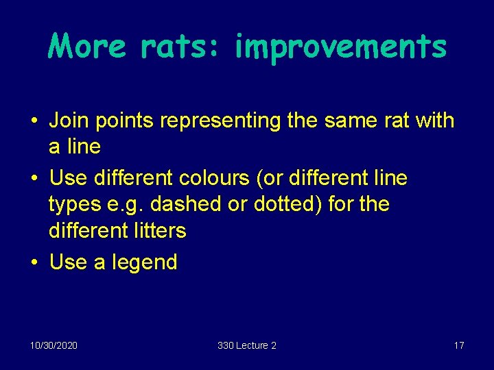
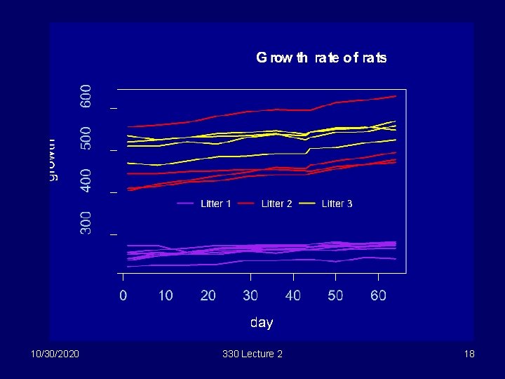
More rats: improvements • Join points representing the same rat with a line • Use different colours (or different line types e. g. dashed or dotted) for the different litters • Use a legend 10/30/2020 330 Lecture 2 17

10/30/2020 330 Lecture 2 18

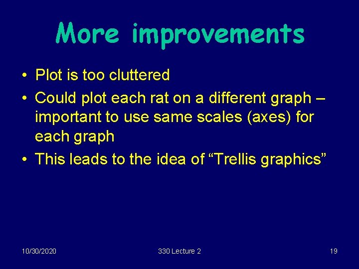
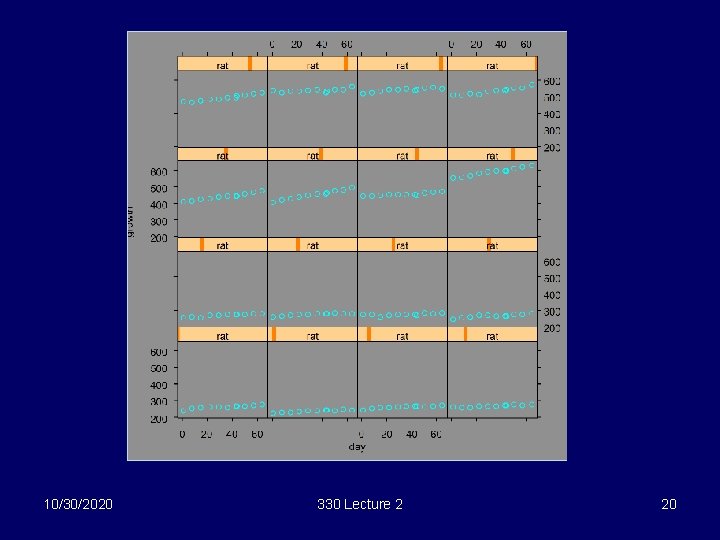
More improvements • Plot is too cluttered • Could plot each rat on a different graph – important to use same scales (axes) for each graph • This leads to the idea of “Trellis graphics” 10/30/2020 330 Lecture 2 19

10/30/2020 330 Lecture 2 20

10/30/2020 330 Lecture 2 21

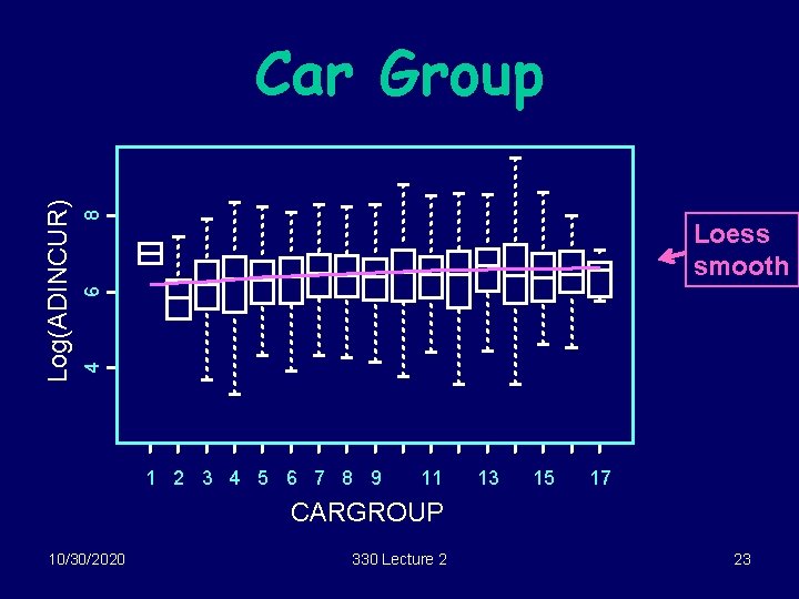
Two variables: one continuous, one categorical • Insurance data: data on 14, 000 insurance claims. Want to explore relationship between the amount of the claim (a continuous variable) and the type of car (a categorical variable). • Use side-by side boxplots. 10/30/2020 330 Lecture 2 22

8 6 Loess smooth 4 Log(ADINCUR) Car Group 1 2 3 4 5 6 7 8 9 11 13 15 17 CARGROUP 10/30/2020 330 Lecture 2 23

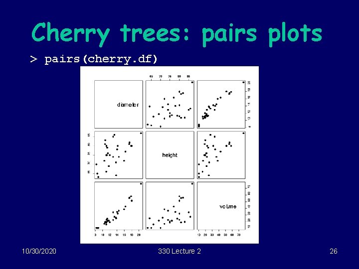
More than 2 variables: • If all variables are continuous, we can explore the relationships between them using a pairs plot • If we have 3 variables, a rotating plot is a very useful tool 10/30/2020 330 Lecture 2 24

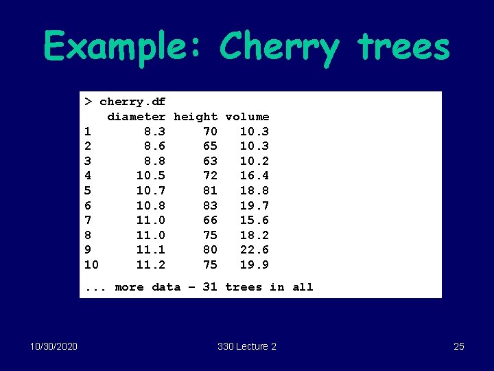
Example: Cherry trees > cherry. df diameter height volume 1 8. 3 70 10. 3 2 8. 6 65 10. 3 3 8. 8 63 10. 2 4 10. 5 72 16. 4 5 10. 7 81 18. 8 6 10. 8 83 19. 7 7 11. 0 66 15. 6 8 11. 0 75 18. 2 9 11. 1 80 22. 6 10 11. 2 75 19. 9. . . more data – 31 trees in all 10/30/2020 330 Lecture 2 25

Cherry trees: pairs plots > pairs(cherry. df) 10/30/2020 330 Lecture 2 26

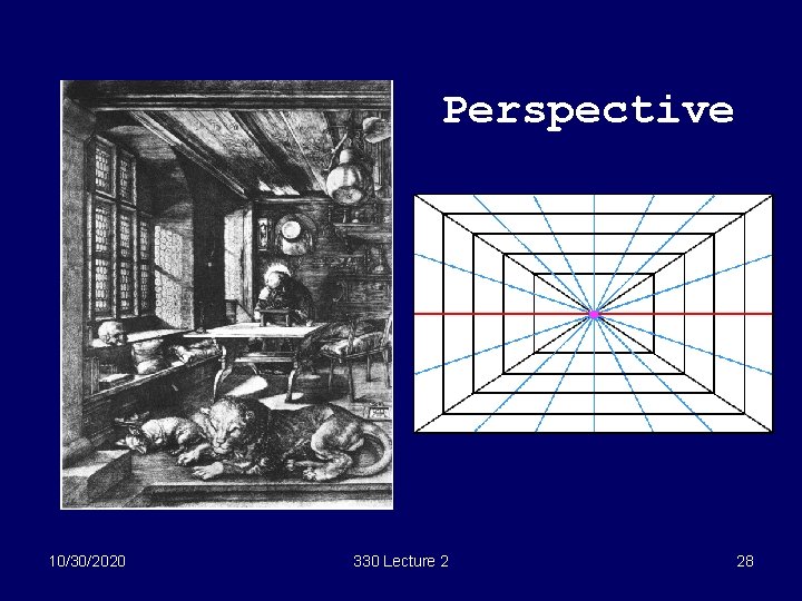
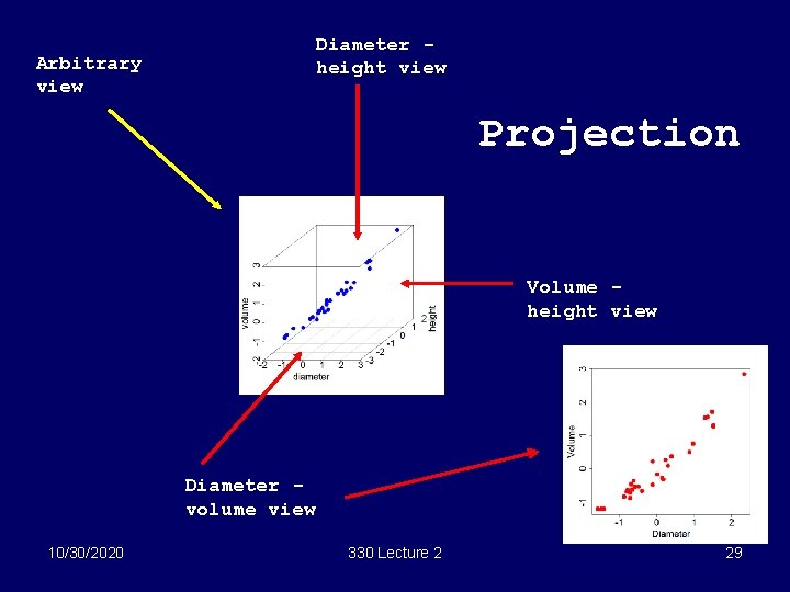
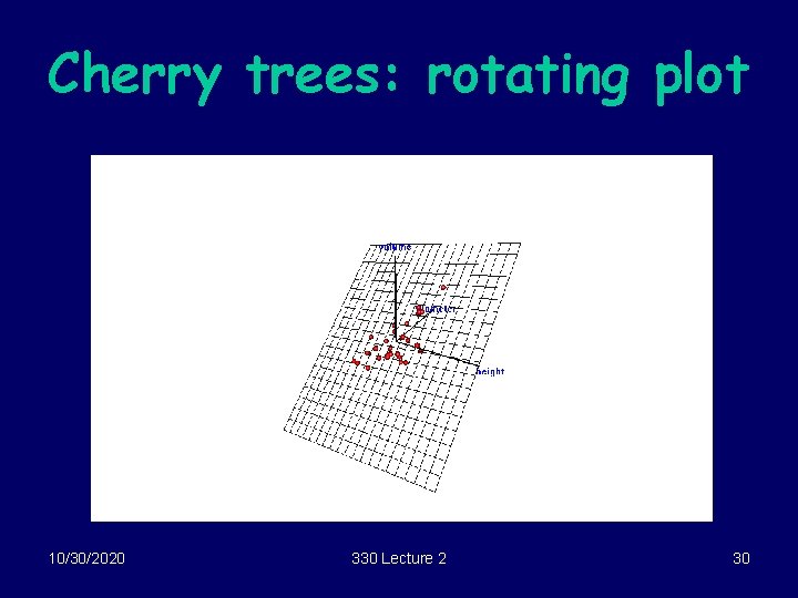
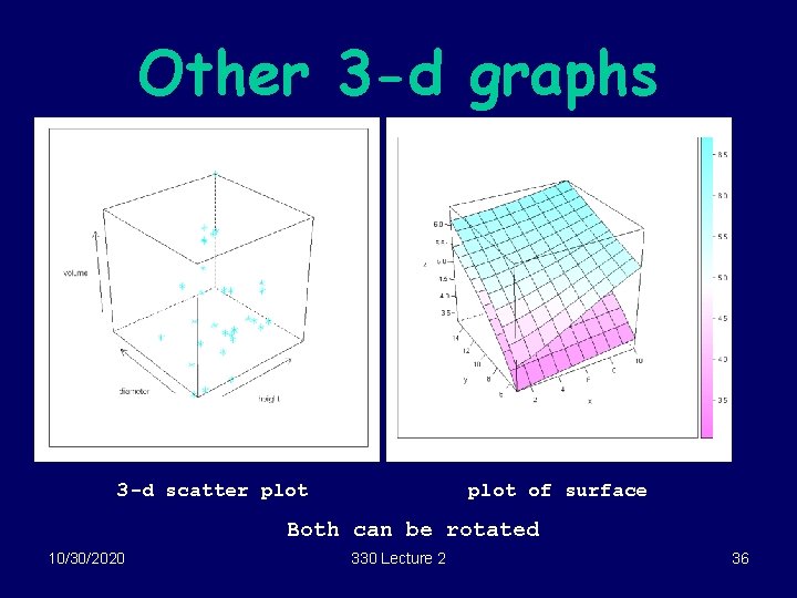
3 -d Rotating plots • The challenge: to represent a 3 dimensional object on a 2 -dimensional surface (a TV screen, computer screen etc) • Traditional method uses projection, perspective • A powerful idea is to use motion, looking at the 3 -d scene from different angles 10/30/2020 330 Lecture 2 27

Perspective 10/30/2020 330 Lecture 2 28

Diameter height view Arbitrary view Projection Volume height view Diameter volume view 10/30/2020 330 Lecture 2 29

Cherry trees: rotating plot 10/30/2020 330 Lecture 2 30

Dynamic motion • By dynamically changing the angle of view, we get a better impression of the 3 dimensional structure of the data • “Dynamic graphics” is a very powerful tool 10/30/2020 330 Lecture 2 31

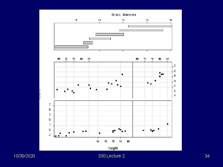
A powerful idea: Coplots • Coplot shows relationship between x and y for selected values of z (usually a narrow range of z’s) • By showing separate plots for different z ranges, we can see how the relationship between x and y changes as z changes • Coplot: conditioning plot, shows relationship between x and y conditional on z (ie for fixed z) 10/30/2020 330 Lecture 2 32

Cherry trees: coplots • To show the relationship between height and volume for different values of diameter: • Divide the range of diameter (8. 3 to 20. 6) up into 6 subranges 8 -11, 10. 5 -11. 5 etc • Draw 6 plots, the first using all data whose diameter is between 8 and 11, the second using all data whose diameter is between 10. 5 and 11. 5, and so on 10/30/2020 330 Lecture 2 33

10/30/2020 330 Lecture 2 34

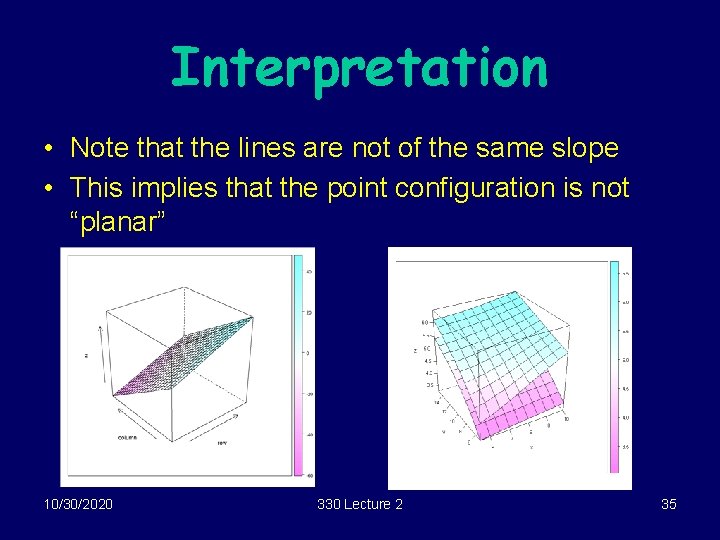
Interpretation • Note that the lines are not of the same slope • This implies that the point configuration is not “planar” 10/30/2020 330 Lecture 2 35

Other 3 -d graphs 3 -d scatter plot of surface Both can be rotated 10/30/2020 330 Lecture 2 36