STATS 330 Lecture 15 12132021 330 lecture 15

STATS 330: Lecture 15 12/13/2021 330 lecture 15 1

Variable selection Aim of today’s lecture § To describe some further techniques for selecting the explanatory variables for a regression § To compare the techniques and apply them to several examples 12/13/2021 330 lecture 15 2

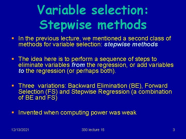
Variable selection: Stepwise methods § In the previous lecture, we mentioned a second class of methods for variable selection: stepwise methods § The idea here is to perform a sequence of steps to eliminate variables from the regression, or add variables to the regression (or perhaps both). § Three variations: Backward Elimination (BE), Forward Selection (FS) and Stepwise Regression (a combination of BE and FS) § Invented when computing power was weak 12/13/2021 330 lecture 15 3

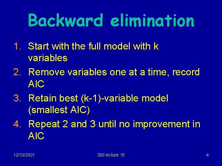
Backward elimination 1. Start with the full model with k variables 2. Remove variables one at a time, record AIC 3. Retain best (k-1)-variable model (smallest AIC) 4. Repeat 2 and 3 until no improvement in AIC 12/13/2021 330 lecture 15 4

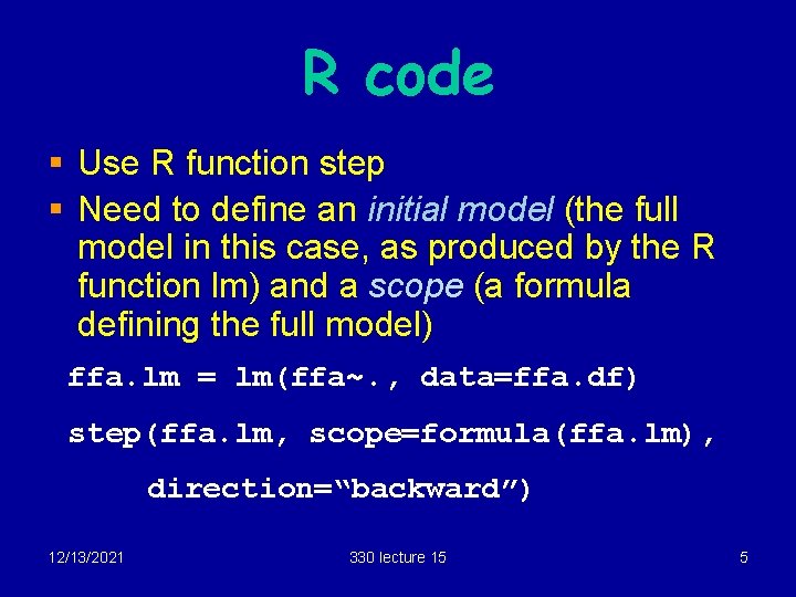
R code § Use R function step § Need to define an initial model (the full model in this case, as produced by the R function lm) and a scope (a formula defining the full model) ffa. lm = lm(ffa~. , data=ffa. df) step(ffa. lm, scope=formula(ffa. lm), direction=“backward”) 12/13/2021 330 lecture 15 5

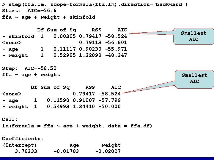
> step(ffa. lm, scope=formula(ffa. lm), direction="backward") Start: AIC=-56. 6 ffa ~ age + weight + skinfold Df Sum of Sq - skinfold 1 0. 00305 <none> - age 1 0. 11117 - weight 1 0. 52985 RSS 0. 79417 0. 79113 0. 90230 1. 32098 AIC -58. 524 -56. 601 -55. 971 -48. 347 Step: AIC=-58. 52 ffa ~ age + weight Df Sum of Sq <none> - age - weight 1 1 RSS AIC 0. 79417 -58. 524 0. 11590 0. 91007 -57. 799 0. 54993 1. 34410 -50. 000 Smallest AIC Call: lm(formula = ffa ~ age + weight, data = ffa. df) Coefficients: (Intercept) 12/13/2021 3. 78333 age -0. 01783 weight 330 lecture 15 -0. 02027 6

Forward selection § Start with a null model § Fit all one-variable models in turn. Pick the model with the best AIC § Then, fit all two variable models that contain the variable selected in 2. Pick the one for which the added variable gives the best AIC § Continue in this way until adding further variables does not improve the AIC 12/13/2021 330 lecture 15 7

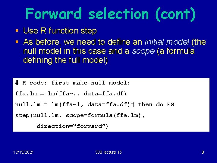
Forward selection (cont) § Use R function step § As before, we need to define an initial model (the null model in this case and a scope (a formula defining the full model) # R code: first make null model: ffa. lm = lm(ffa~. , data=ffa. df) null. lm = lm(ffa~1, data=ffa. df)# then do FS step(null. lm, scope=formula(ffa. lm), direction=“forward”) 12/13/2021 330 lecture 15 8

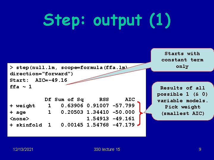
Step: output (1) > step(null. lm, scope=formula(ffa. lm), direction="forward") Start: AIC=-49. 16 ffa ~ 1 Df Sum of Sq RSS AIC + weight 1 0. 63906 0. 91007 -57. 799 + age 1 0. 20503 1. 34410 -50. 000 <none> 1. 54913 -49. 161 + skinfold 1 0. 00145 1. 54768 -47. 179 12/13/2021 330 lecture 15 Starts with constant term only Results of all possible 1 (& 0) variable models. Pick weight (smallest AIC) 9

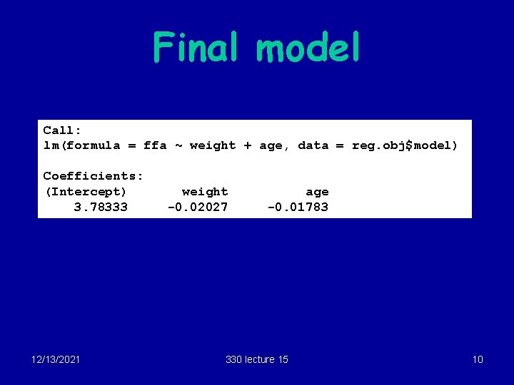
Final model Call: lm(formula = ffa ~ weight + age, data = reg. obj$model) Coefficients: (Intercept) 3. 78333 12/13/2021 weight -0. 02027 age -0. 01783 330 lecture 15 10

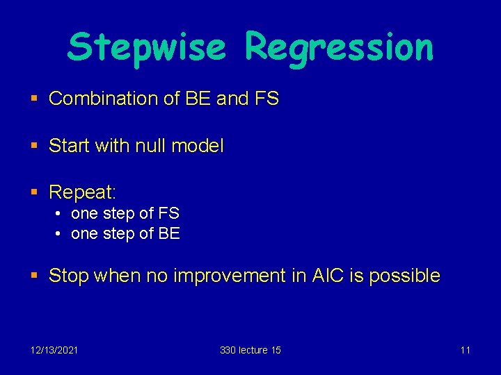
Stepwise Regression § Combination of BE and FS § Start with null model § Repeat: • one step of FS • one step of BE § Stop when no improvement in AIC is possible 12/13/2021 330 lecture 15 11

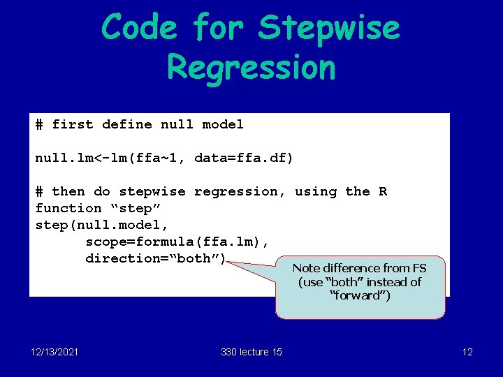
Code for Stepwise Regression # first define null model null. lm<-lm(ffa~1, data=ffa. df) # then do stepwise regression, using the R function “step” step(null. model, scope=formula(ffa. lm), direction=“both”) Note difference from FS (use “both” instead of “forward”) 12/13/2021 330 lecture 15 12

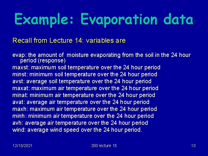
Example: Evaporation data Recall from Lecture 14: variables are evap: the amount of moisture evaporating from the soil in the 24 hour period (response) maxst: maximum soil temperature over the 24 hour period minst: minimum soil temperature over the 24 hour period avst: average soil temperature over the 24 hour period maxat: maximum air temperature over the 24 hour period minat: minimum air temperature over the 24 hour period avat: average air temperature over the 24 hour period maxh: maximum air temperature over the 24 hour period minh: minimum air temperature over the 24 hour period avh: average air temperature over the 24 hour period wind: average wind speed over the 24 hour period. 12/13/2021 330 lecture 15 13

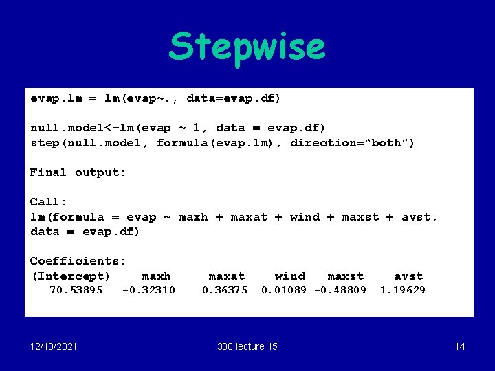
Stepwise evap. lm = lm(evap~. , data=evap. df) null. model<-lm(evap ~ 1, data = evap. df) step(null. model, formula(evap. lm), direction=“both”) Final output: Call: lm(formula = evap ~ maxh + maxat + wind + maxst + avst, data = evap. df) Coefficients: (Intercept) 70. 53895 12/13/2021 maxh -0. 32310 maxat 0. 36375 wind maxst avst 0. 01089 -0. 48809 1. 19629 330 lecture 15 14

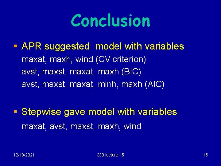
Conclusion § APR suggested model with variables maxat, maxh, wind (CV criterion) avst, maxat, maxh (BIC) avst, maxat, minh, maxh (AIC) § Stepwise gave model with variables maxat, avst, maxh, wind 12/13/2021 330 lecture 15 15

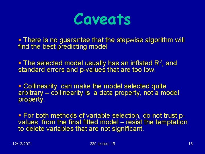
Caveats § There is no guarantee that the stepwise algorithm will find the best predicting model § The selected model usually has an inflated R 2, and standard errors and p-values that are too low. § Collinearity can make the model selected quite arbitrary – collinearity is a data property, not a model property. § For both methods of variable selection, do not trust pvalues from the final fitted model – resist the temptation to delete variables that are not significant. 12/13/2021 330 lecture 15 16

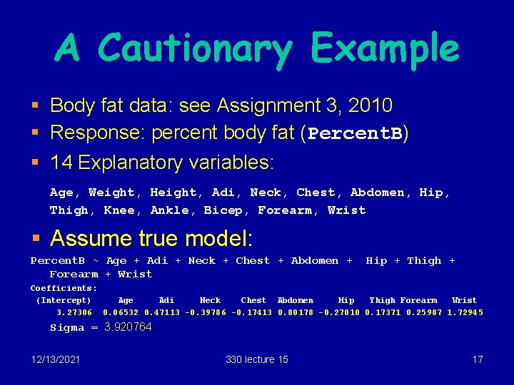
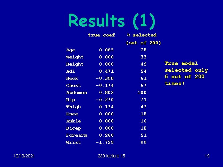
A Cautionary Example § Body fat data: see Assignment 3, 2010 § Response: percent body fat (Percent. B) § 14 Explanatory variables: Age, Weight, Height, Adi, Neck, Chest, Abdomen, Hip, Thigh, Knee, Ankle, Bicep, Forearm, Wrist § Assume true model: Percent. B ~ Age + Adi + Neck + Chest + Abdomen + Forearm + Wrist Hip + Thigh + Coefficients: (Intercept) Age Adi Neck Chest Abdomen Hip Thigh Forearm Wrist 3. 27306 0. 06532 0. 47113 -0. 39786 -0. 17413 0. 80178 -0. 27010 0. 17371 0. 25987 1. 72945 Sigma = 3. 920764 12/13/2021 330 lecture 15 17

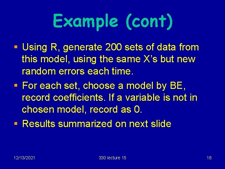
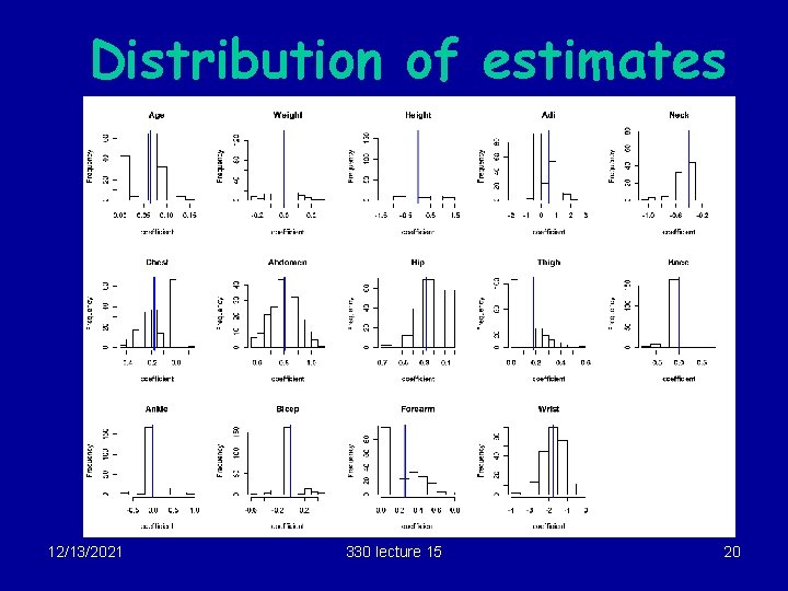
Example (cont) § Using R, generate 200 sets of data from this model, using the same X’s but new random errors each time. § For each set, choose a model by BE, record coefficients. If a variable is not in chosen model, record as 0. § Results summarized on next slide 12/13/2021 330 lecture 15 18

Results (1) true coef Age Weight Height Adi Neck Chest Abdomen Hip Thigh Knee Ankle Bicep Forearm Wrist 12/13/2021 0. 065 0. 000 0. 471 -0. 398 -0. 174 0. 802 -0. 270 0. 174 0. 000 0. 260 -1. 729 330 lecture 15 % selected (out of 200) 78 33 True model 42 selected only 54 6 out of 200 61 times! 67 100 71 47 18 16 18 51 99 19

Distribution of estimates 12/13/2021 330 lecture 15 20

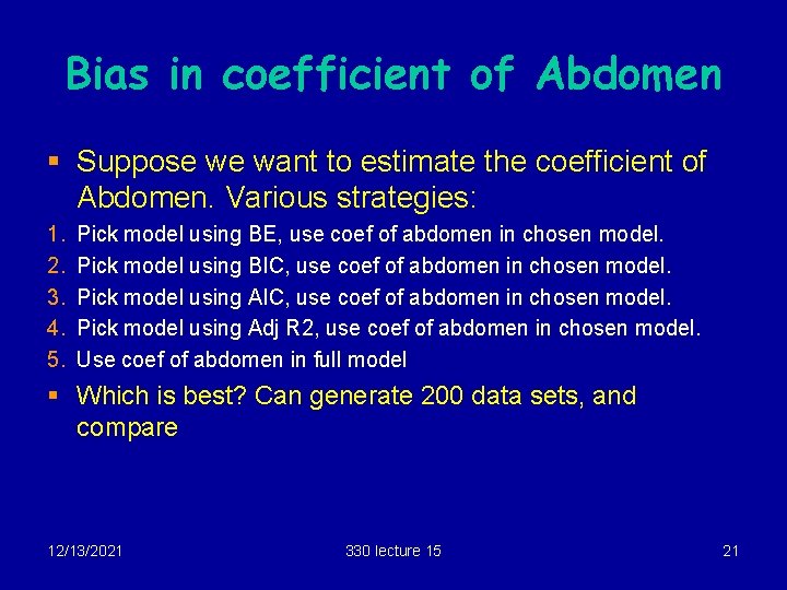
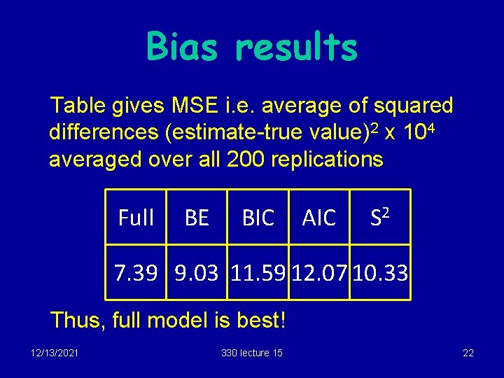
Bias in coefficient of Abdomen § Suppose we want to estimate the coefficient of Abdomen. Various strategies: 1. 2. 3. 4. 5. Pick model using BE, use coef of abdomen in chosen model. Pick model using BIC, use coef of abdomen in chosen model. Pick model using Adj R 2, use coef of abdomen in chosen model. Use coef of abdomen in full model § Which is best? Can generate 200 data sets, and compare 12/13/2021 330 lecture 15 21

Bias results Table gives MSE i. e. average of squared differences (estimate-true value)2 x 104 averaged over all 200 replications Full BE BIC AIC S 2 7. 39 9. 03 11. 59 12. 07 10. 33 Thus, full model is best! 12/13/2021 330 lecture 15 22

Estimating the “optimism” in R 2 § We noted (caveats slide 16) that the R 2 for the selected model is usually higher than the R 2 for the model fitted to new data. § How can we adjust for this? § If we have plenty of data, we can split the data into a “training set” and a “test set”, select the model using the training set, then calculate the R 2 for the test set. 12/13/2021 330 lecture 15 23

Example: the Georgia voting data § In the 2000 US presidential election, some voters had their ballots declared invalid for different reasons. § In this data set, the response is the “undercount” (the difference between the votes cast and the votes declared valid). § Each observation is a Georgia county, of which there were 159. We removed 4 outliers, leaving 155 counties. § We will consider a model with 5 explanatory variables: undercount ~ per. AA+rural+gore+bush+other § Data is in the faraway package 12/13/2021 330 lecture 15 24

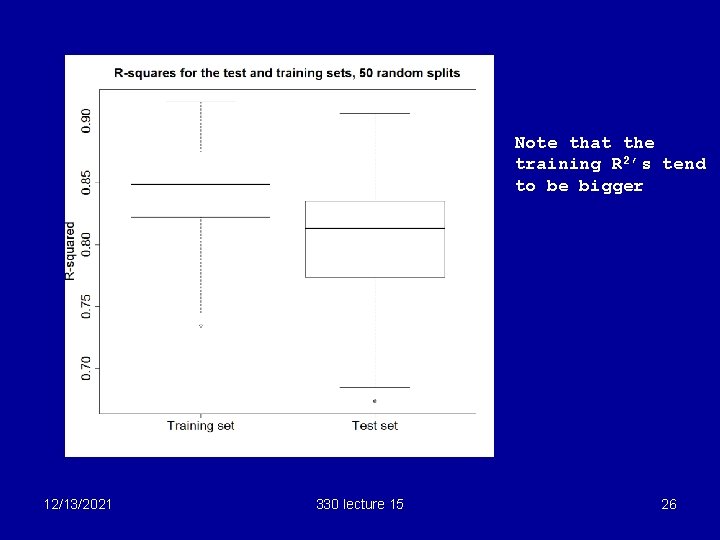
Calculating the optimism § We split the data into 2 parts at random, a training set of 80 and a test set of 75. § Using the training set, we selected a model using stepwise regression and calculated the R 2. § We then took the chosen model and recalculated the R 2 using the test set. The difference is the “optimism” § We repeated for 50 random splits of 80/75, getting 50 training set R 2’s and 50 test set R 2’s. § Boxplots of these are shown next 12/13/2021 330 lecture 15 25

Note that the training R 2’s tend to be bigger 12/13/2021 330 lecture 15 26

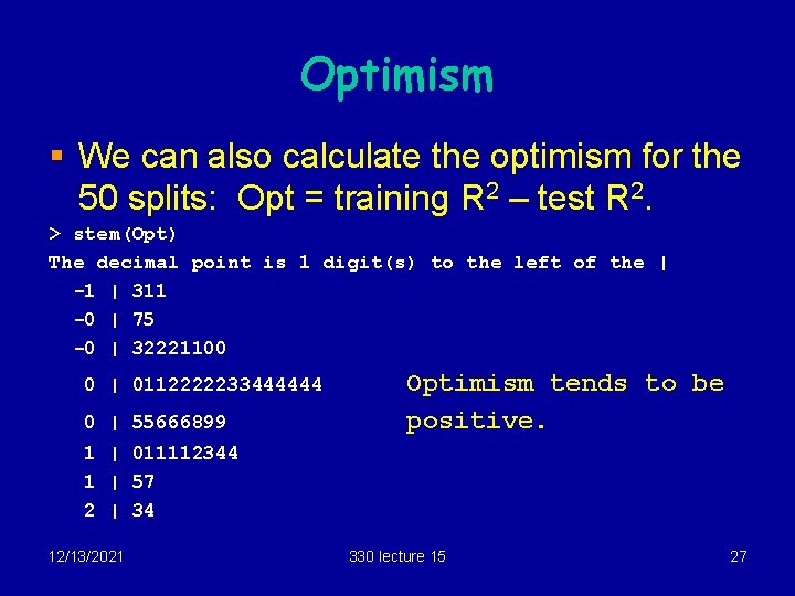
Optimism § We can also calculate the optimism for the 50 splits: Opt = training R 2 – test R 2. > stem(Opt) The decimal point is 1 digit(s) to the left of the | -1 | 311 -0 | 75 -0 | 32221100 0 | 0112222233444444 0 | 55666899 Optimism tends to be positive. 1 | 011112344 1 | 57 2 | 34 12/13/2021 330 lecture 15 27

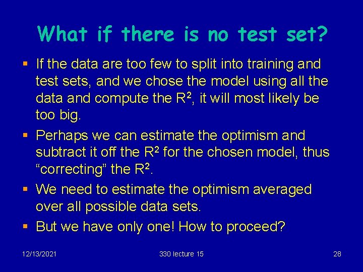
What if there is no test set? § If the data are too few to split into training and test sets, and we chose the model using all the data and compute the R 2, it will most likely be too big. § Perhaps we can estimate the optimism and subtract it off the R 2 for the chosen model, thus “correcting” the R 2. § We need to estimate the optimism averaged over all possible data sets. § But we have only one! How to proceed? 12/13/2021 330 lecture 15 28

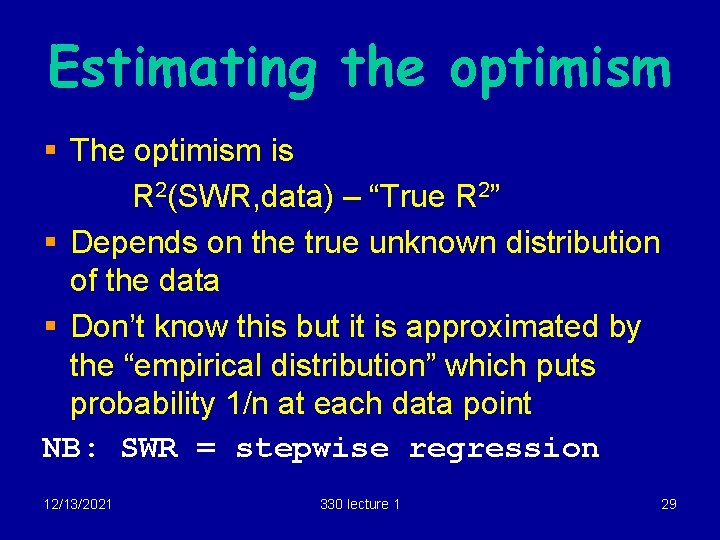
Estimating the optimism § The optimism is R 2(SWR, data) – “True R 2” § Depends on the true unknown distribution of the data § Don’t know this but it is approximated by the “empirical distribution” which puts probability 1/n at each data point NB: SWR = stepwise regression 12/13/2021 330 lecture 1 29

Resampling § We can draw a sample from the empirical distribution by choosing a sample of size n chosen at random with replacement from the original data (n= number of observations in the original data). § Also called a “bootstrap sample” or a “resample” 12/13/2021 330 lecture 15 30

“Empirical optimism” § The “empirical optimism” is R 2(SWR, resampled data) – R 2(SWR, original data) § We can generate as many values of this estimate as we like by repeatedly drawing samples from the empirical distribution, or “resampling” 12/13/2021 330 lecture 15 31

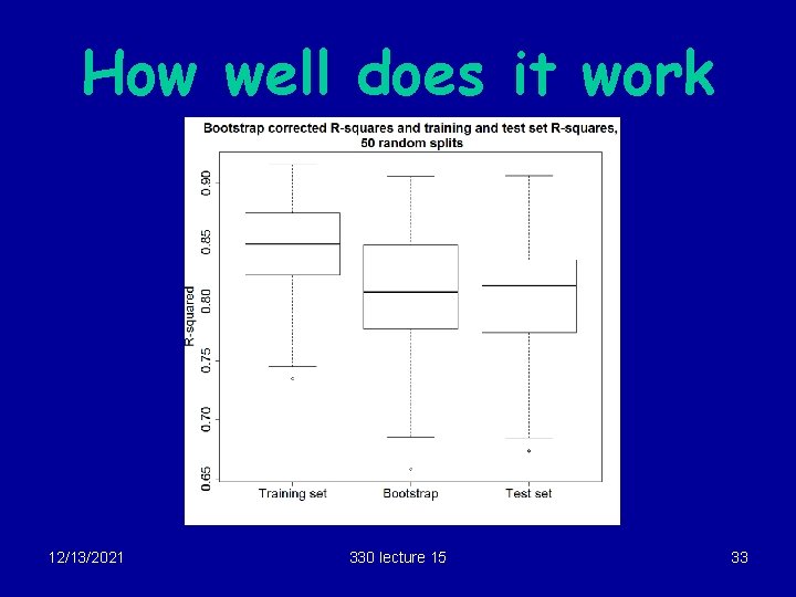
Resampling (cont) To correct the R 2: § Compute the empirical optimism § Repeat for say 200 resamples, average the 200 optimisms. § This is our estimated optimism. § Correct the original R 2 for the chosen model by subtracting off the estimated optimism. § This is the “bootstrap corrected” R 2. 12/13/2021 330 lecture 15 32

How well does it work 12/13/2021 330 lecture 15 33

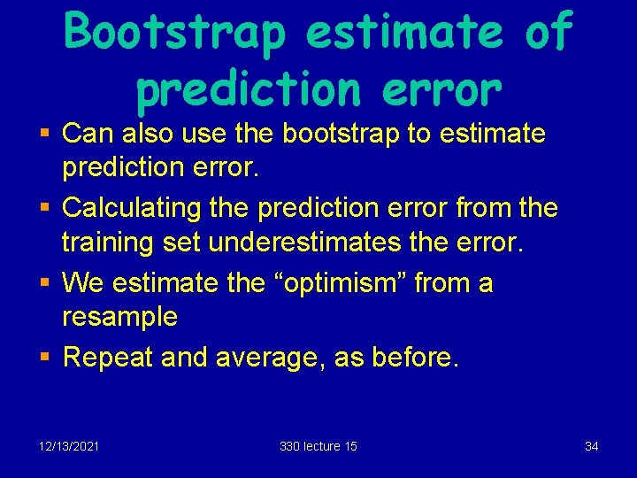
Bootstrap estimate of prediction error § Can also use the bootstrap to estimate prediction error. § Calculating the prediction error from the training set underestimates the error. § We estimate the “optimism” from a resample § Repeat and average, as before. 12/13/2021 330 lecture 15 34

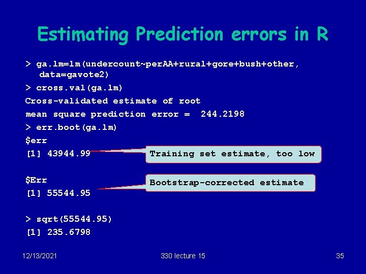
Estimating Prediction errors in R > ga. lm=lm(undercount~per. AA+rural+gore+bush+other, data=gavote 2) > cross. val(ga. lm) Cross-validated estimate of root mean square prediction error = 244. 2198 > err. boot(ga. lm) $err [1] 43944. 99 Training set estimate, too low $Err [1] 55544. 95 Bootstrap-corrected estimate > sqrt(55544. 95) [1] 235. 6798 12/13/2021 330 lecture 15 35

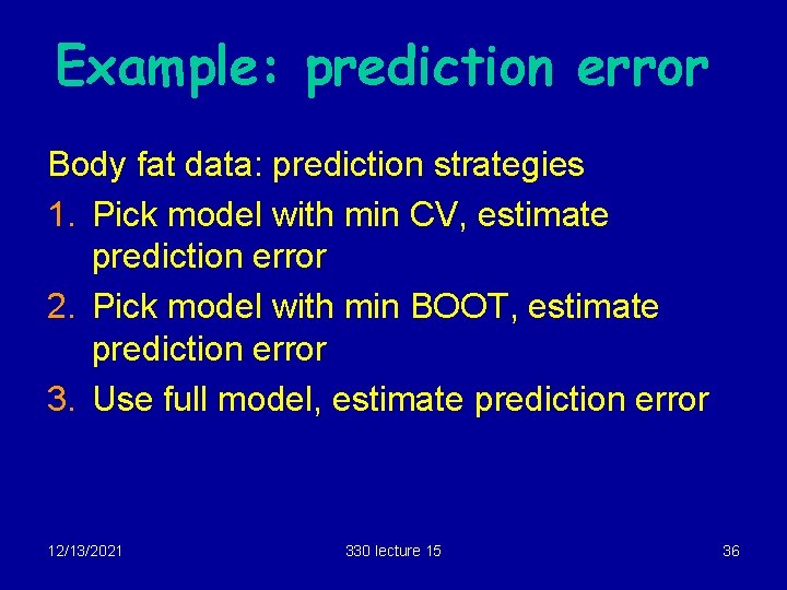
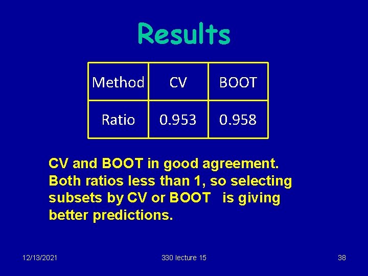
Example: prediction error Body fat data: prediction strategies 1. Pick model with min CV, estimate prediction error 2. Pick model with min BOOT, estimate prediction error 3. Use full model, estimate prediction error 12/13/2021 330 lecture 15 36

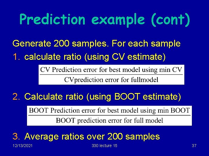
Prediction example (cont) Generate 200 samples. For each sample 1. calculate ratio (using CV estimate) 2. Calculate ratio (using BOOT estimate) 3. Average ratios over 200 samples 12/13/2021 330 lecture 15 37

Results Method CV BOOT Ratio 0. 953 0. 958 CV and BOOT in good agreement. Both ratios less than 1, so selecting subsets by CV or BOOT is giving better predictions. 12/13/2021 330 lecture 15 38