STATS 330 Lecture 8 1222020 330 lecture 8

STATS 330: Lecture 8 12/2/2020 330 lecture 8 1

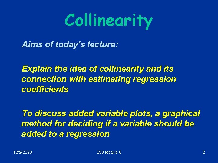
Collinearity Aims of today’s lecture: Explain the idea of collinearity and its connection with estimating regression coefficients To discuss added variable plots, a graphical method for deciding if a variable should be added to a regression 12/2/2020 330 lecture 8 2

Variance of regression coefficients § We saw in Lecture 6 how the standard errors of the regression coefficients depend on the error variance s 2: the bigger s 2, the bigger the standard errors. § We also suggested that the standard error depends on the arrangement of the x’s. § In today’s lecture, we explore this idea a bit further. 12/2/2020 330 lecture 8 3

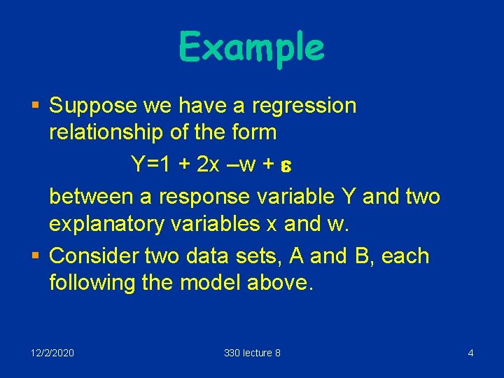
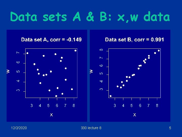
Example § Suppose we have a regression relationship of the form Y=1 + 2 x –w + e between a response variable Y and two explanatory variables x and w. § Consider two data sets, A and B, each following the model above. 12/2/2020 330 lecture 8 4

Data sets A & B: x, w data 12/2/2020 330 lecture 8 5

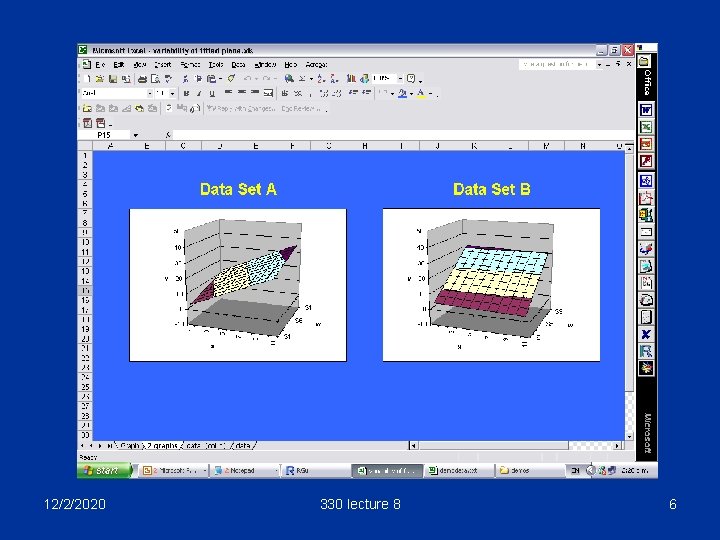
12/2/2020 330 lecture 8 6

Conclusion: § The greater the correlation, the more variable the plane. § In fact, for the coefficient b of x 12/2/2020 330 lecture 8 7

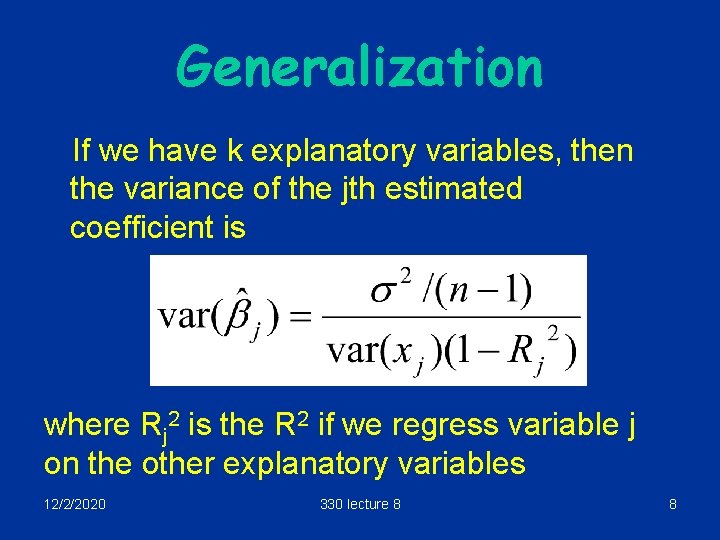
Generalization If we have k explanatory variables, then the variance of the jth estimated coefficient is where Rj 2 is the R 2 if we regress variable j on the other explanatory variables 12/2/2020 330 lecture 8 8

Best case § If xj is orthogonal to (uncorrelated with) the other explanatory variables, then Rj 2 is zero and the variance is the smallest possible i. e. 12/2/2020 330 lecture 8 9

Variance inflation factor The factor represents the increase in variance caused by correlation between the explanatory variables and is called the variance inflation factor (VIF) 12/2/2020 330 lecture 8 10

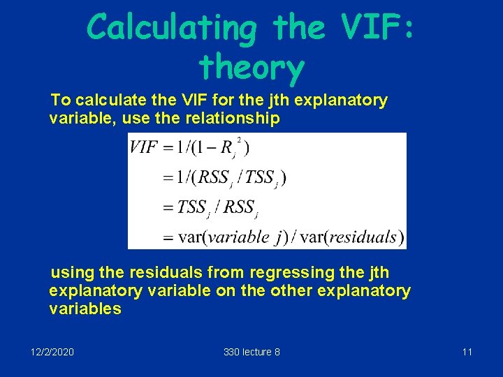
Calculating the VIF: theory To calculate the VIF for the jth explanatory variable, use the relationship using the residuals from regressing the jth explanatory variable on the other explanatory variables 12/2/2020 330 lecture 8 11

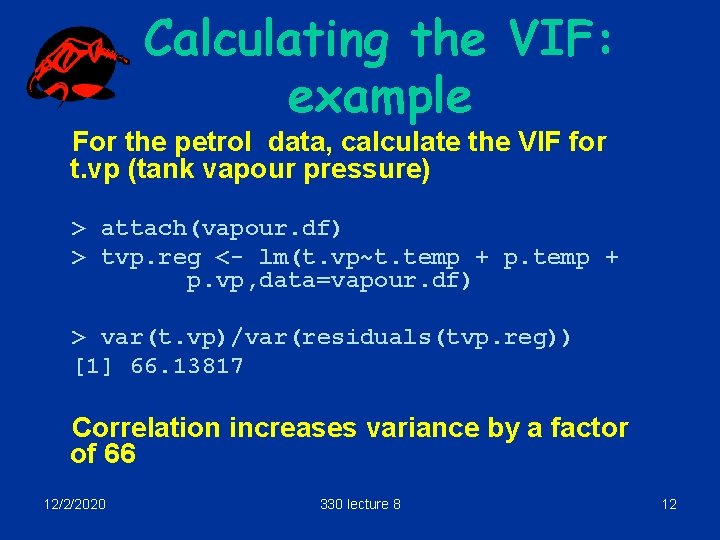
Calculating the VIF: example For the petrol data, calculate the VIF for t. vp (tank vapour pressure) > attach(vapour. df) > tvp. reg <- lm(t. vp~t. temp + p. vp, data=vapour. df) > var(t. vp)/var(residuals(tvp. reg)) [1] 66. 13817 Correlation increases variance by a factor of 66 12/2/2020 330 lecture 8 12

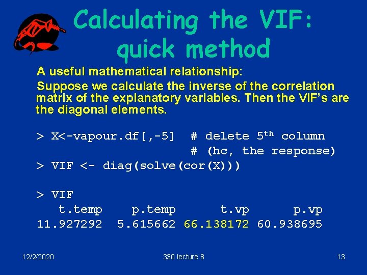
Calculating the VIF: quick method A useful mathematical relationship: Suppose we calculate the inverse of the correlation matrix of the explanatory variables. Then the VIF’s are the diagonal elements. # delete 5 th column # (hc, the response) > VIF <- diag(solve(cor(X))) > X<-vapour. df[, -5] > VIF t. temp 11. 927292 12/2/2020 p. temp t. vp p. vp 5. 615662 66. 138172 60. 938695 330 lecture 8 13

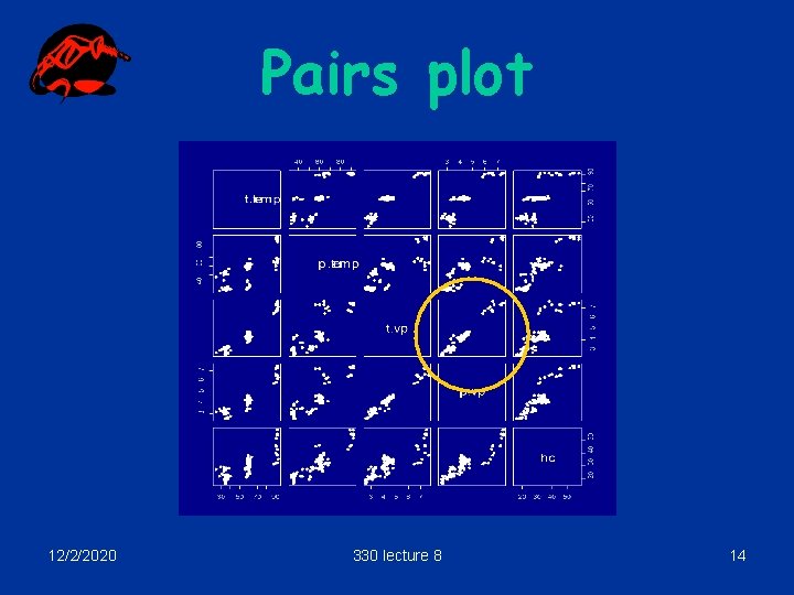
Pairs plot 12/2/2020 330 lecture 8 14

Collinearity § If one or more variables in a regression have big VIF’s, the regression is said to be collinear § Caused by one or more variables being almost linear combinations of the others § Sometimes indicated by high correlations between the independent variables § Results in imprecise estimation of regression coefficients § Standard errors are high, so t-statistics are small, variables are often non-significant ( data is insufficient to detect a difference) 12/2/2020 330 lecture 8 15

Non-significance § If a variable has a non-significant t, then either • The variable is not related to the response, or • The variable is related to the response, but it is not required in the regression because it is strongly related to a third variable that is in the regression, so we don’t need both. § First case: small t-value, small VIF, small correlation with response § Second case, small t-value, big VIF, big correlation with response 12/2/2020 330 lecture 8 16

Remedy § The usual remedy is to drop one or more variables from the model. § This “breaks” the linear relationship between the variables § This leads to the problem of “subset selection”, which subset to choose. § See Lectures 14 and 15 12/2/2020 330 lecture 8 17

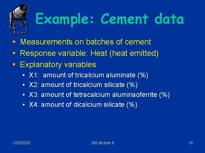
Example: Cement data § Measurements on batches of cement § Response variable: Heat (heat emitted) § Explanatory variables • • X 1: amount of tricalcium aluminate (%) X 2: amount of tricalcium silicate (%) X 3: amount of tetracalcium aluminaoferrite (%) X 4: amount of dicalcium silicate (%) 12/2/2020 330 lecture 8 18

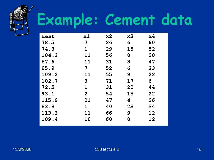
Example: Cement data Heat 78. 5 74. 3 104. 3 87. 6 95. 9 109. 2 102. 7 72. 5 93. 1 115. 9 83. 8 113. 3 109. 4 12/2/2020 X 1 7 1 11 11 7 11 3 1 2 21 1 11 10 X 2 26 29 56 31 52 55 71 31 54 47 40 66 68 330 lecture 8 X 3 6 15 8 8 6 9 17 22 18 4 23 9 8 X 4 60 52 20 47 33 22 6 44 22 26 34 12 12 19

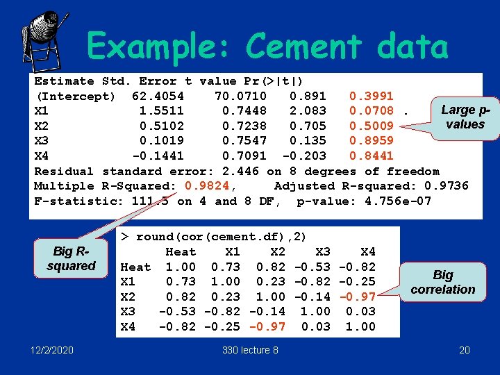
Example: Cement data Estimate Std. Error t value Pr(>|t|) (Intercept) 62. 4054 70. 0710 0. 891 0. 3991 Large p. X 1 1. 5511 0. 7448 2. 083 0. 0708. values X 2 0. 5102 0. 7238 0. 705 0. 5009 X 3 0. 1019 0. 7547 0. 135 0. 8959 X 4 -0. 1441 0. 7091 -0. 203 0. 8441 Residual standard error: 2. 446 on 8 degrees of freedom Multiple R-Squared: 0. 9824, Adjusted R-squared: 0. 9736 F-statistic: 111. 5 on 4 and 8 DF, p-value: 4. 756 e-07 Big Rsquared 12/2/2020 > round(cor(cement. df), 2) Heat X 1 X 2 X 3 X 4 Heat 1. 00 0. 73 0. 82 -0. 53 -0. 82 X 1 0. 73 1. 00 0. 23 -0. 82 -0. 25 X 2 0. 82 0. 23 1. 00 -0. 14 -0. 97 X 3 -0. 53 -0. 82 -0. 14 1. 00 0. 03 X 4 -0. 82 -0. 25 -0. 97 0. 03 1. 00 330 lecture 8 Big correlation 20

Cement data > diag(solve(cor(cement. df[, -1]))) X 1 X 2 X 3 38. 49621 254. 42317 Omit Heat X 4 46. 86839 282. 51286 Very large! cement. df$X 1 + cement. df$X 2 + cement. df$X 3 + cement. df$X 4 [1] 99 97 95 97 98 97 97 98 96 98 98 12/2/2020 330 lecture 8 21

Drop X 4 > diag(solve(cor(cement. df[, -c(1, 5)]))) X 1 X 2 X 3 3. 251068 1. 063575 3. 142125 VIF’s now small Estimate Std. Error t value Pr(>|t|) (Intercept) 48. 19363 3. 91330 12. 315 6. 17 e-07 *** X 1 1. 69589 0. 20458 8. 290 1. 66 e-05 *** X 2 0. 65691 0. 04423 14. 851 1. 23 e-07 *** X 3 0. 25002 0. 18471 1. 354 0. 209 X 1, X 2 now signif Residual standard error: 2. 312 on 9 degrees of freedom Multiple R-Squared: 0. 9823, Adjusted R-squared: 0. 9764 F-statistic: 166. 3 on 3 and 9 DF, p-value: 3. 367 e-08 12/2/2020 330 lecture 8 22

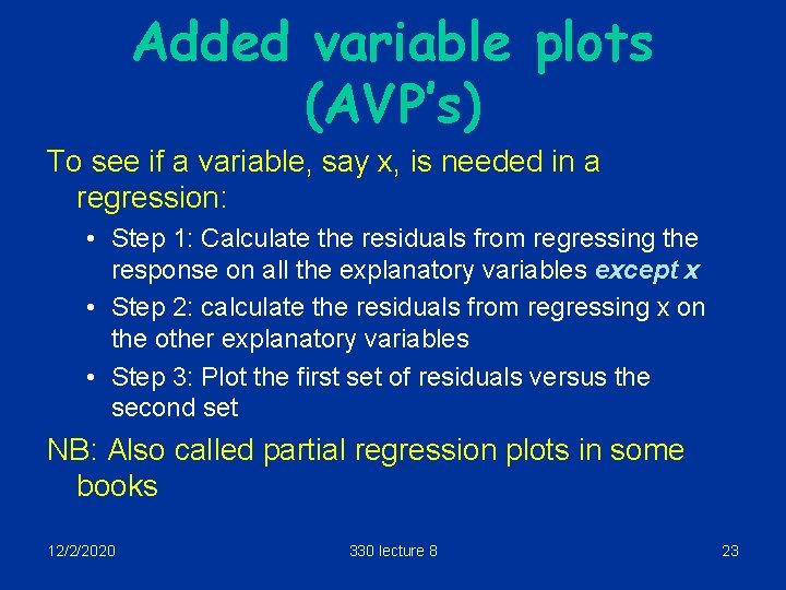
Added variable plots (AVP’s) To see if a variable, say x, is needed in a regression: • Step 1: Calculate the residuals from regressing the response on all the explanatory variables except x • Step 2: calculate the residuals from regressing x on the other explanatory variables • Step 3: Plot the first set of residuals versus the second set NB: Also called partial regression plots in some books 12/2/2020 330 lecture 8 23

Rationale § The first set of residuals represents the variation in y not explained by the other explanatory variables § The second set of residuals represents the part of x not explained by the other explanatory variables § If there is a relationship between the two sets, there is a relationship between x and the response that is not accounted for by the other explanatory variables § Thus, if we see a relationship in the plot, x is needed in the regression!!! 12/2/2020 330 lecture 8 24

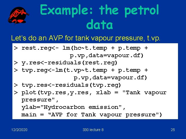
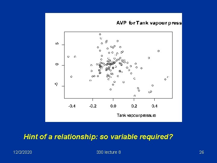
Example: the petrol data Let’s do an AVP for tank vapour pressure, t. vp. > rest. reg<- lm(hc~t. temp + p. vp, data=vapour. df) > y. res<-residuals(rest. reg) > tvp. reg<-lm(t. vp~t. temp + p. vp, data=vapour. df) > tvp. res<-residuals(tvp. reg) > plot(tvp. res, y. res, xlab = "Tank vapour pressure", ylab="Hydrocarbon emission", main = “AVP for Tank vapour pressure") 12/2/2020 330 lecture 8 25

Hint of a relationship: so variable required? 12/2/2020 330 lecture 8 26

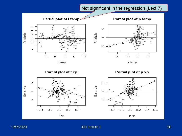
Short cut in R There is a function added. variable. plots in R to draw the plots automatically. This is one of the functions in the R 330 package which must be installed before the function can be used. Note this useful trick! > vapour. lm<-lm(hc~. , data=vapour. df) > par(mfrow=c(2, 2)) # 2 x 2 array of plots > added. variable. plots(vapour. lm) 12/2/2020 330 lecture 8 27

Not significant in the regression (Lect 7) 12/2/2020 330 lecture 8 28

Some curious facts about AVP’s § Assuming a constant term in both regressions, a least squares line fitted though the AVP goes through the origin. § The slope of this line is the fitted regression coefficient for the variable in the original regression § The residuals from this line are the same as the residuals from the original regression 12/2/2020 330 lecture 8 29