Probability Statistics Thomas Schwarz SJ Overview Statistics is

Probability & Statistics Thomas Schwarz, SJ

Overview • Statistics is the lifeblood of data science • • You need to learn how to use statistics But the calculations are implemented in two powerful Python modules • • scipy. statsmodels

Probability • We concentrate on categorical data • Categorical data is discrete: e. g. "not infected", "infected, but no symptoms", "sick", "recovered", "dead" • Categorical data can be ordinal : • • number of cases in Milwaukee County Categorical data can be nominal : • Republican, Democrat, Other, Non-affiliated

Probability Distributions for Categorical Data • Binomial distribution: • Given a binary characteristic (yes/no) and a sample / population of what is the probability that have the characteristics • If we assume that the presence of the characteristic in one individual is independent of the characteristic of another individual

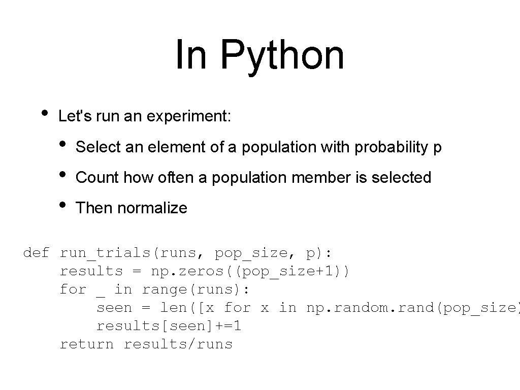
In Python • Let's run an experiment: • • • Select an element of a population with probability p Count how often a population member is selected Then normalize def run_trials(runs, pop_size, p): results = np. zeros((pop_size+1)) for _ in range(runs): seen = len([x for x in np. random. rand(pop_size) results[seen]+=1 return results/runs

In Python • Then compare with the binomial probability • binom. pmf is the probability mass function from scipy. stats import binom results = run_trials(runs, pop_size, p) xvalues = np. arange(0, len(results)) binom. pmf(xvalues, pop_size, p)

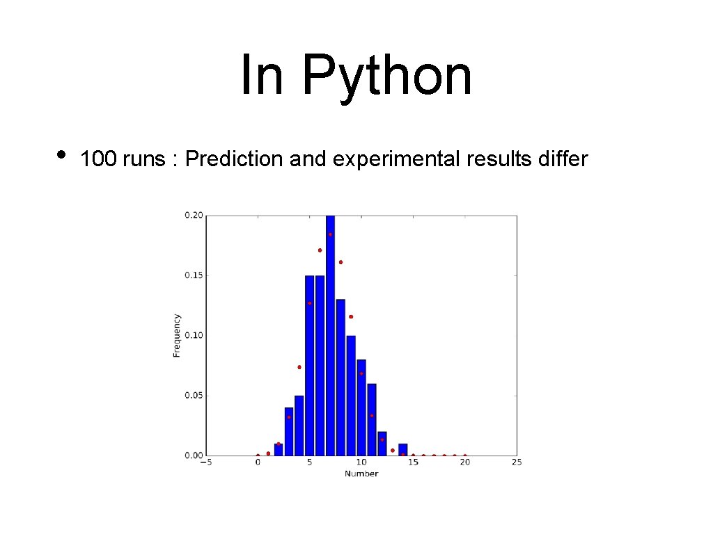
In Python • 100 runs : Prediction and experimental results differ

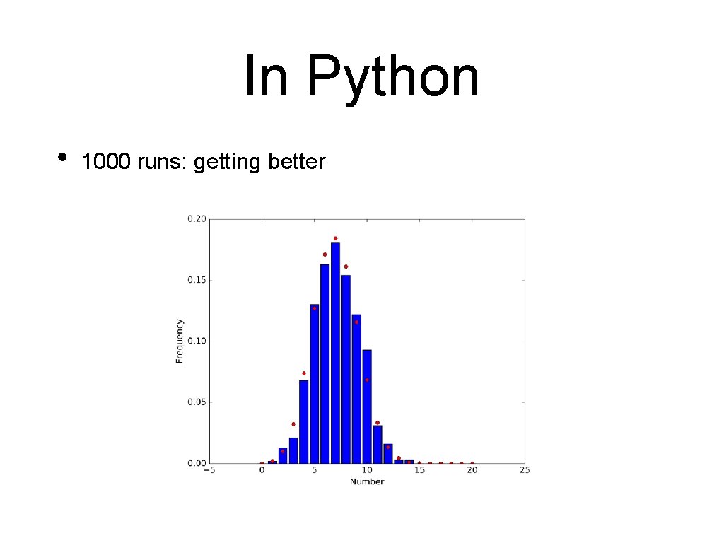
In Python • 1000 runs: getting better

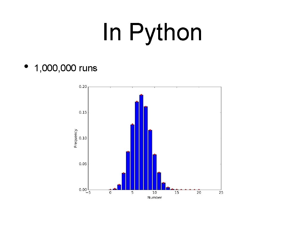
In Python • 1, 000 runs

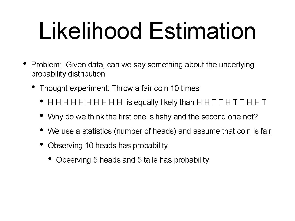
Likelihood Estimation • Problem: Given data, can we say something about the underlying probability distribution • Thought experiment: Throw a fair coin 10 times • • H H H H H is equally likely than H H T T H H T Why do we think the first one is fishy and the second one not? We use a statistics (number of heads) and assume that coin is fair Observing 10 heads has probability • Observing 5 heads and 5 tails has probability

Likelihood Estimation • Reversely • • Given a sample and a putative probability Likelihood: • What is the probability given to observe a statistics on the sample

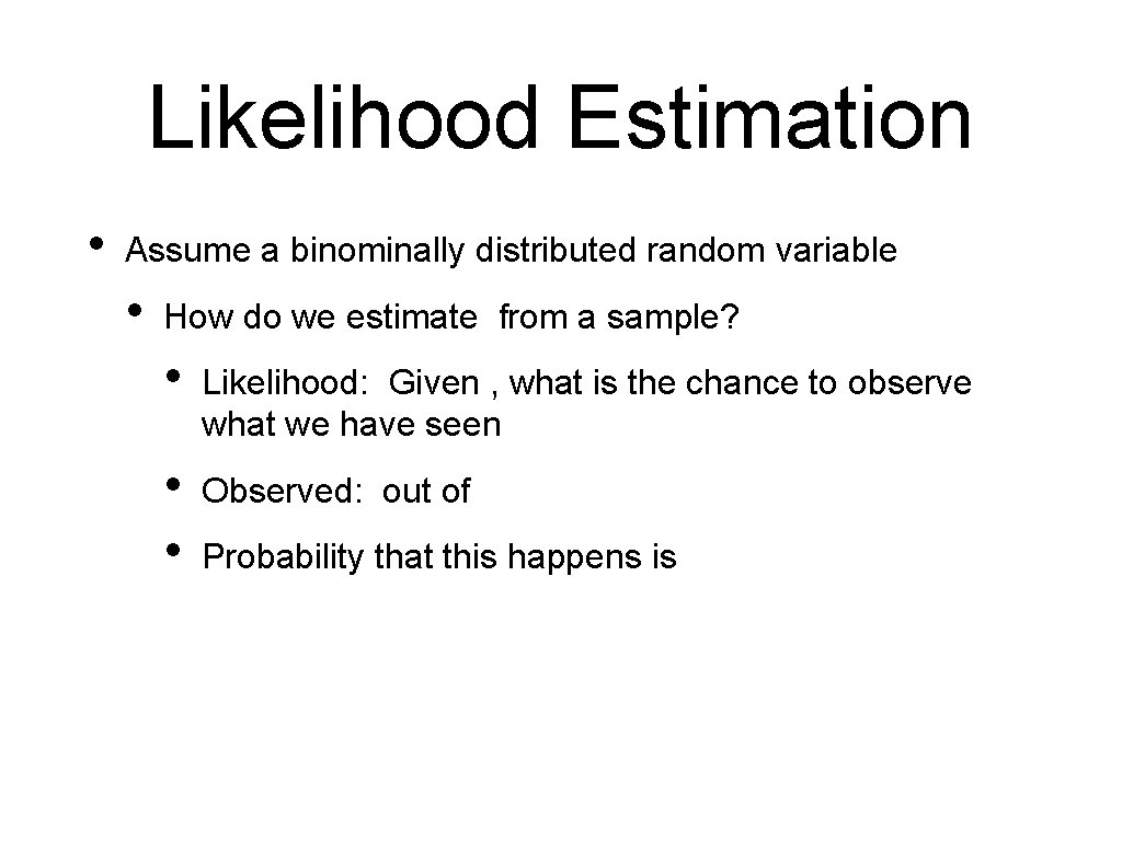
Likelihood Estimation • Assume a binominally distributed random variable • How do we estimate from a sample? • Likelihood: Given , what is the chance to observe what we have seen • • Observed: out of Probability that this happens is

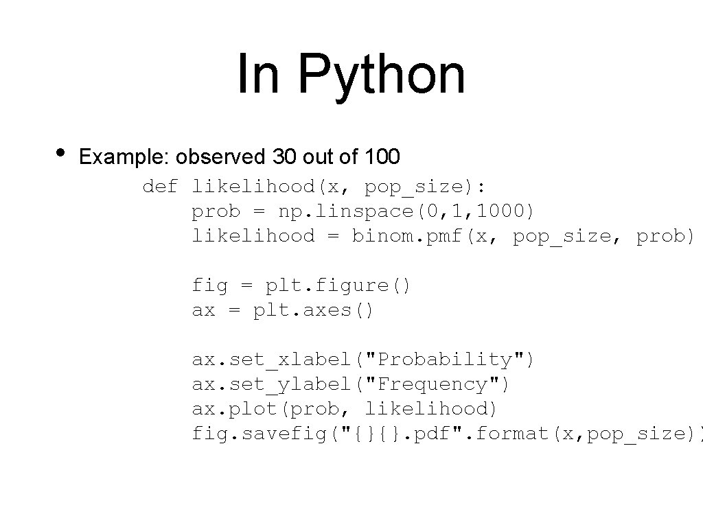
In Python • Example: observed 30 out of 100 def likelihood(x, pop_size): prob = np. linspace(0, 1, 1000) likelihood = binom. pmf(x, pop_size, prob) fig = plt. figure() ax = plt. axes() ax. set_xlabel("Probability") ax. set_ylabel("Frequency") ax. plot(prob, likelihood) fig. savefig("{}{}. pdf". format(x, pop_size))

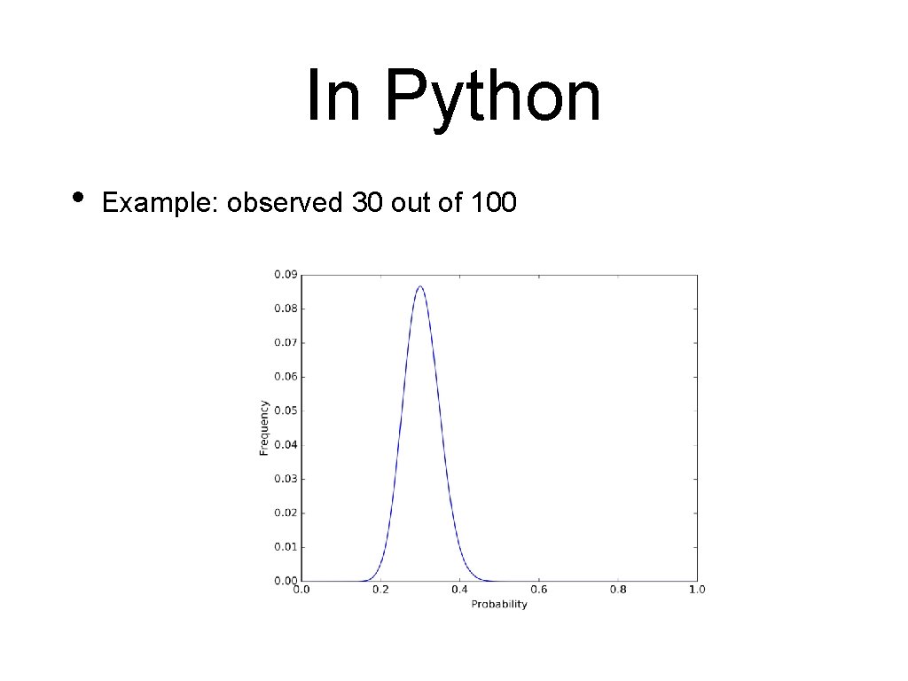
In Python • Example: observed 30 out of 100

Binomial Distribution • • Likelihood is maximized for Formally: • which implies by differentiation that

Binomial Distribution • Therefore: Maximum Likelihood estimator for given out of observations is

Getting Statistics

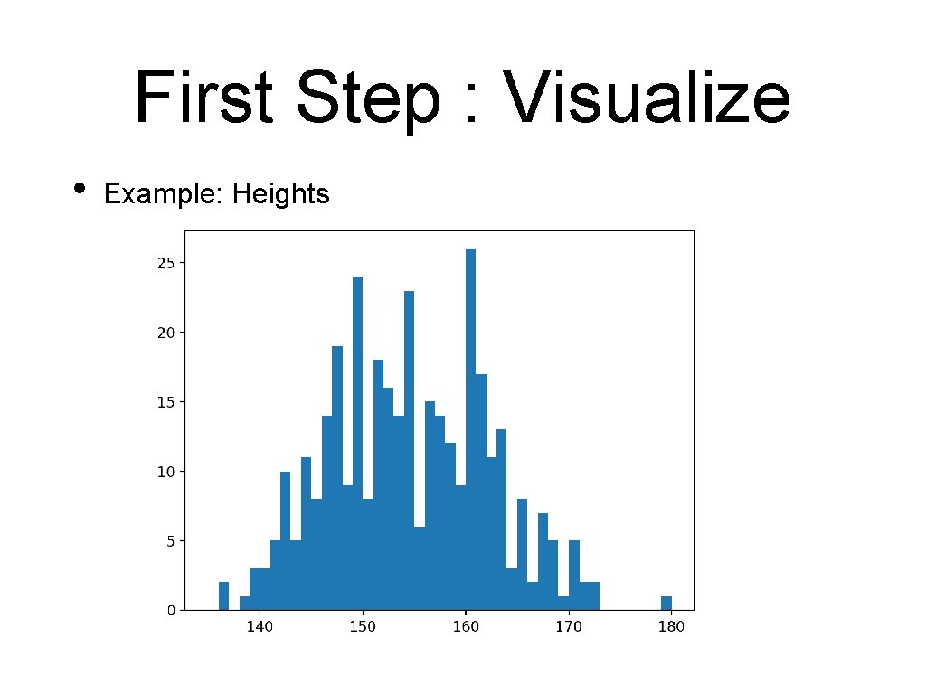
First Step : Visualize • Example: Heights

Second Step: Get Stats • • • Statistic: any type of measure taken on a sample Implemented in scipy. stats Random number generation in np. random

Sample Generation • Use np. random • Returns samples for many different distributions • E. g. • np. random. normal(mean, • np. random. gamma(shape, std, size=1000) scale, size=1000) • Can use numpy. random. seed(12345)to insure same behavior

Getting Statistical Measures • • Use scipy. stats Has many different distributions • scipy. stats. norm is a distribution object • Has a pdf, a cdf, …

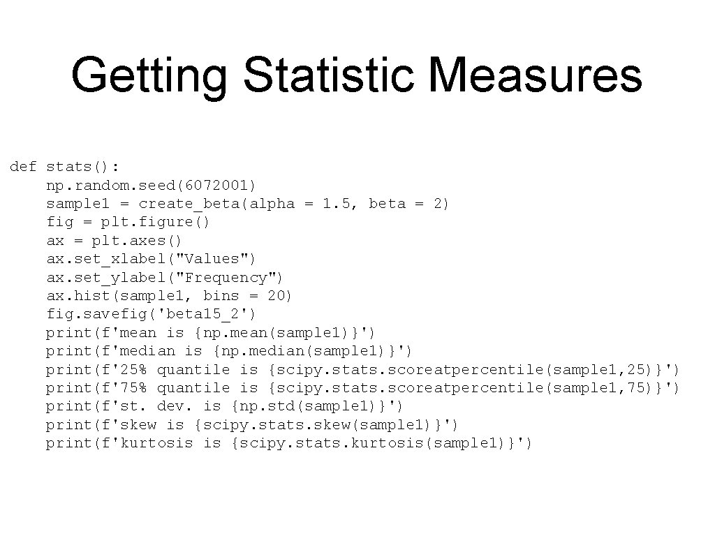
Getting Statistic Measures def stats(): np. random. seed(6072001) sample 1 = create_beta(alpha = 1. 5, beta = 2) fig = plt. figure() ax = plt. axes() ax. set_xlabel("Values") ax. set_ylabel("Frequency") ax. hist(sample 1, bins = 20) fig. savefig('beta 15_2') print(f'mean is {np. mean(sample 1)}') print(f'median is {np. median(sample 1)}') print(f'25% quantile is {scipy. stats. scoreatpercentile(sample 1, 25)}') print(f'75% quantile is {scipy. stats. scoreatpercentile(sample 1, 75)}') print(f'st. dev. is {np. std(sample 1)}') print(f'skew is {scipy. stats. skew(sample 1)}') print(f'kurtosis is {scipy. stats. kurtosis(sample 1)}')

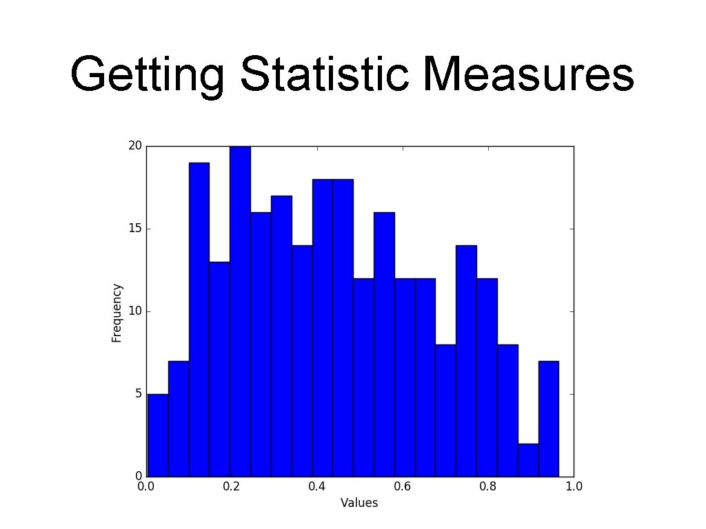
Getting Statistic Measures

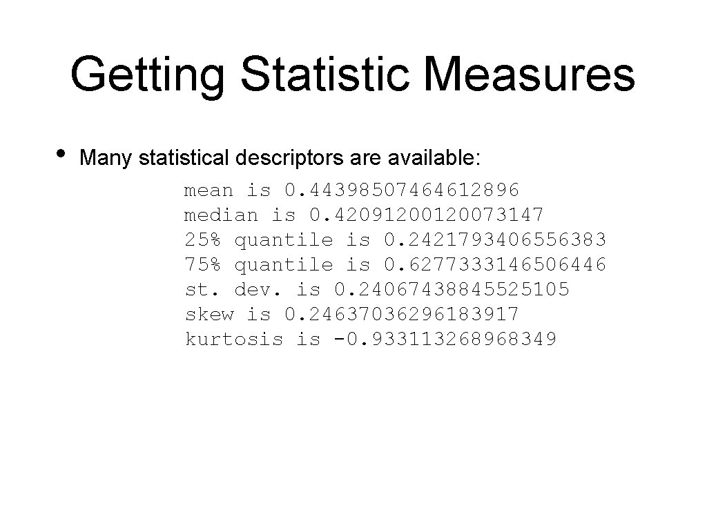
Getting Statistic Measures • Many statistical descriptors are available: mean is 0. 44398507464612896 median is 0. 4209120073147 25% quantile is 0. 2421793406556383 75% quantile is 0. 6277333146506446 st. dev. is 0. 24067438845525105 skew is 0. 24637036296183917 kurtosis is -0. 933113268968349

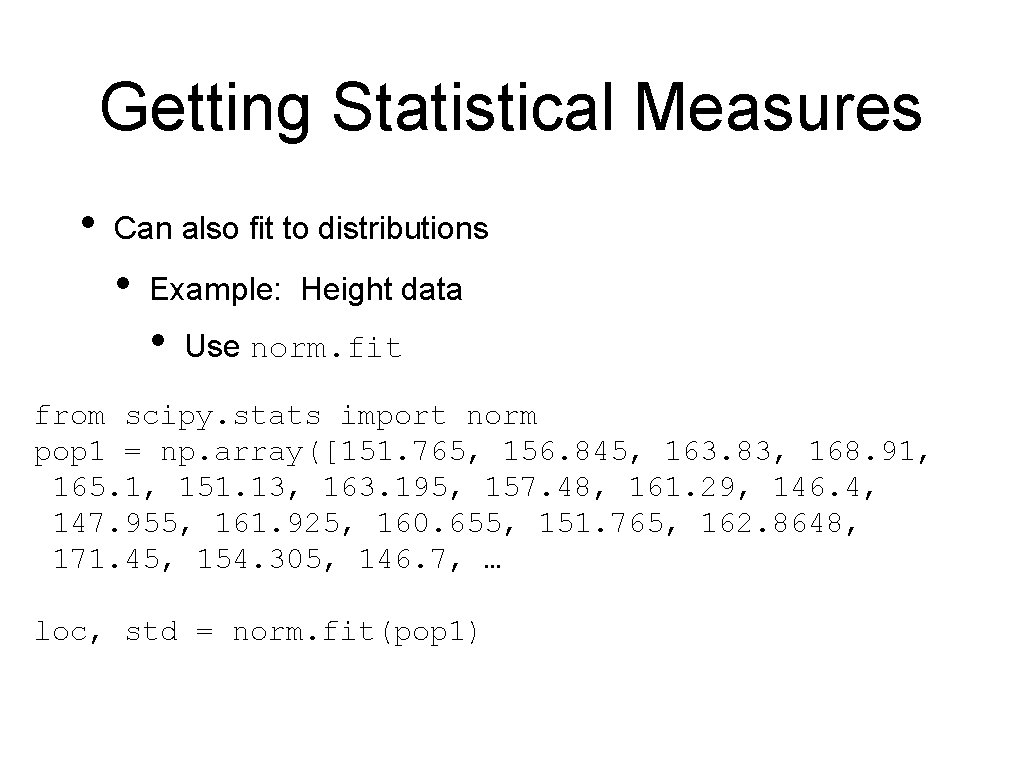
Getting Statistical Measures • Can also fit to distributions • Example: Height data • Use norm. fit from scipy. stats import norm pop 1 = np. array([151. 765, 156. 845, 163. 83, 168. 91, 165. 1, 151. 13, 163. 195, 157. 48, 161. 29, 146. 4, 147. 955, 161. 925, 160. 655, 151. 765, 162. 8648, 171. 45, 154. 305, 146. 7, … loc, std = norm. fit(pop 1)

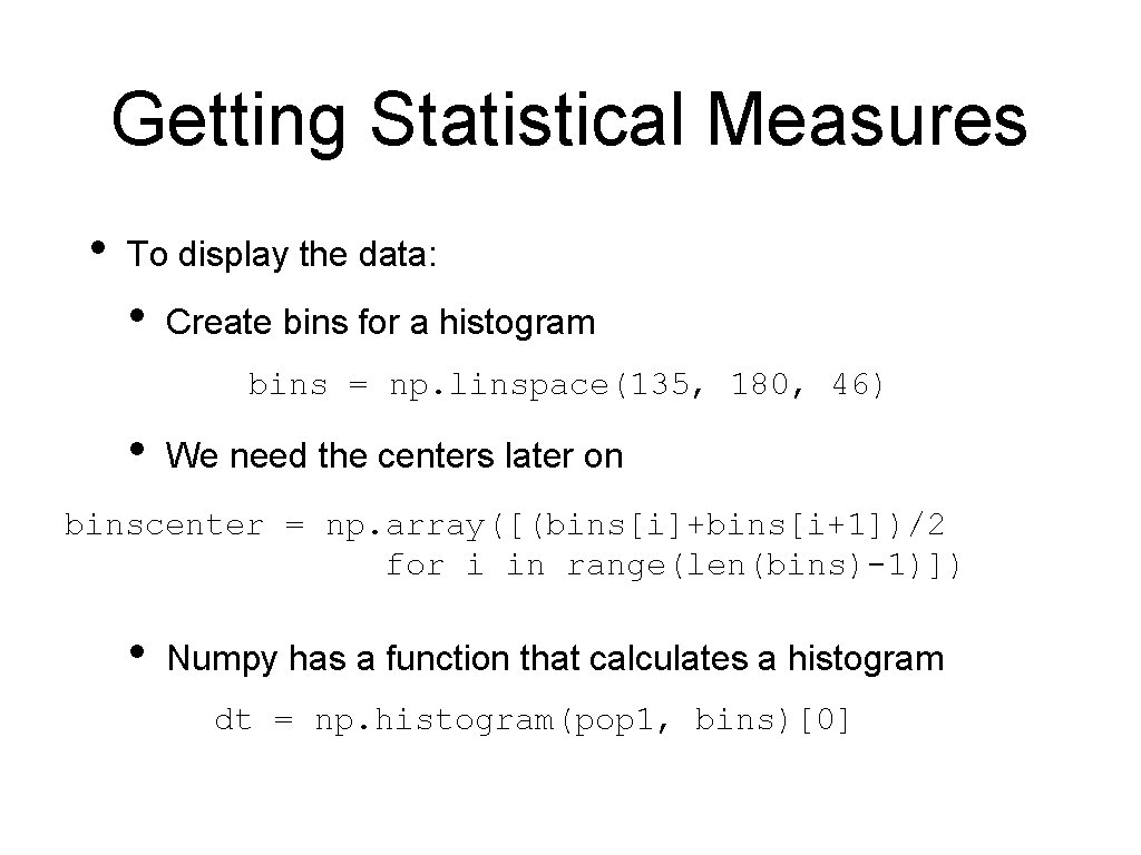
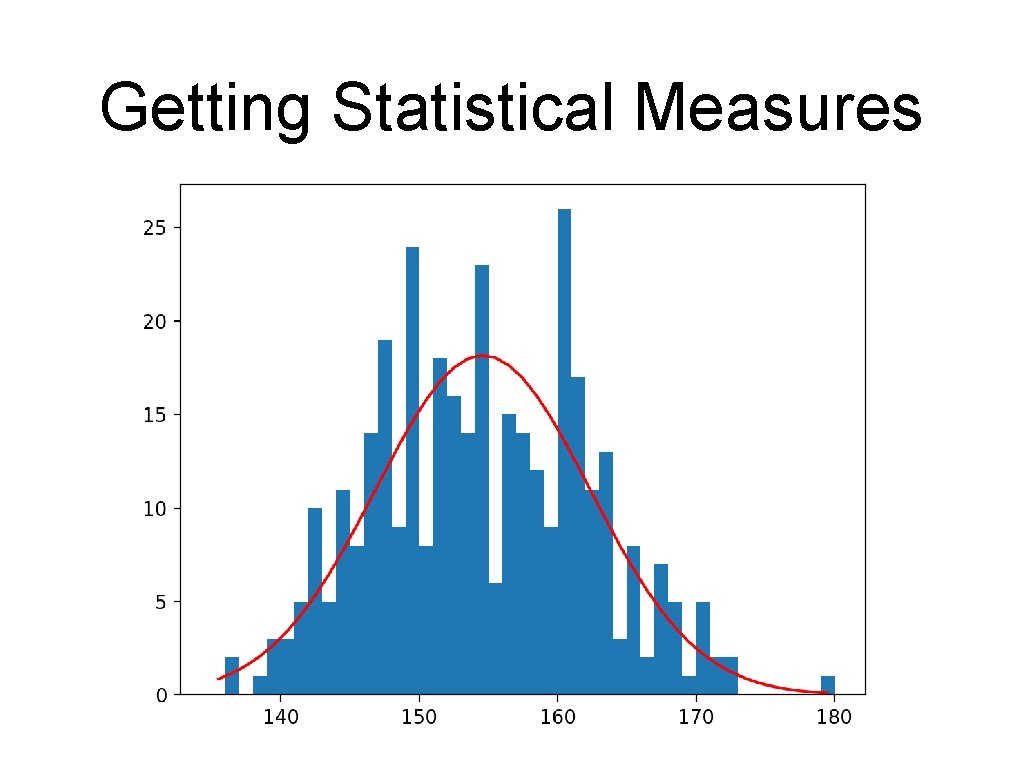
Getting Statistical Measures • To display the data: • Create bins for a histogram bins = np. linspace(135, 180, 46) • We need the centers later on binscenter = np. array([(bins[i]+bins[i+1])/2 for i in range(len(bins)-1)]) • Numpy has a function that calculates a histogram dt = np. histogram(pop 1, bins)[0]

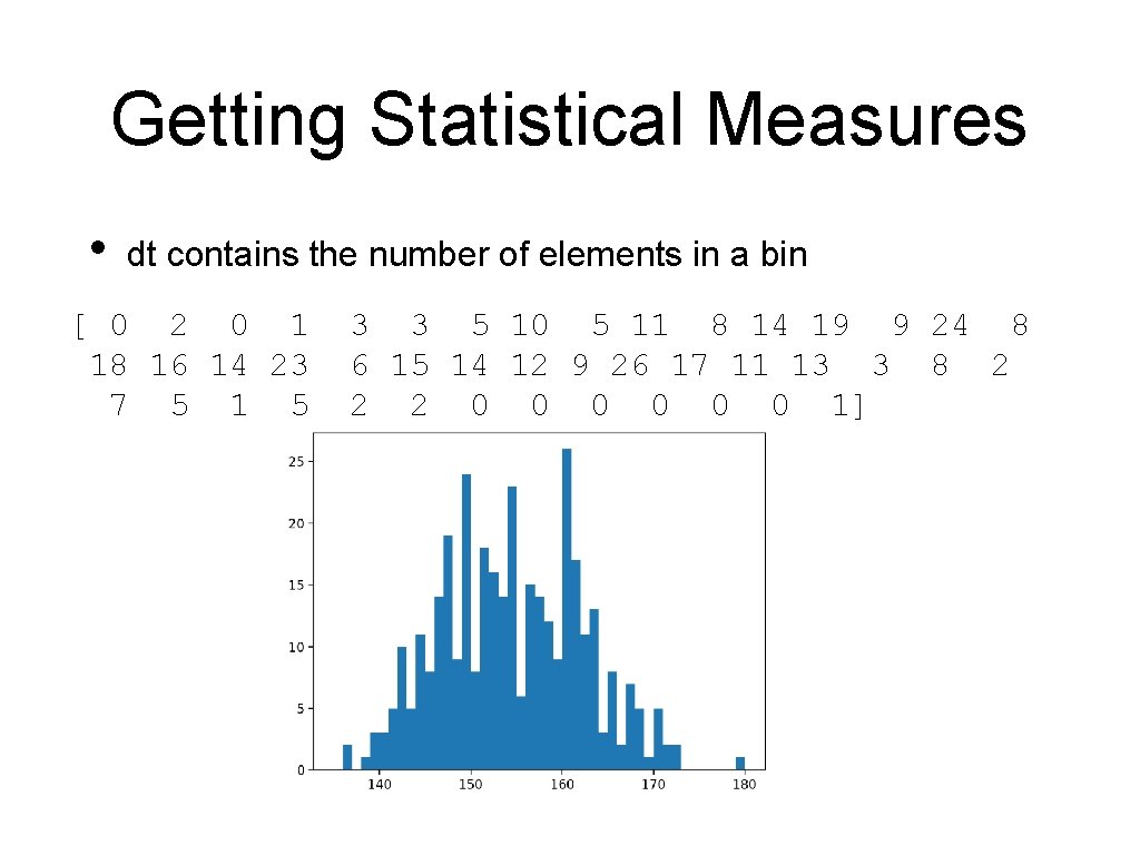
Getting Statistical Measures • dt contains the number of elements in a bin [ 0 2 0 1 18 16 14 23 7 5 1 5 3 3 5 10 5 11 8 14 19 9 24 8 6 15 14 12 9 26 17 11 13 3 8 2 2 2 0 0 0 1]

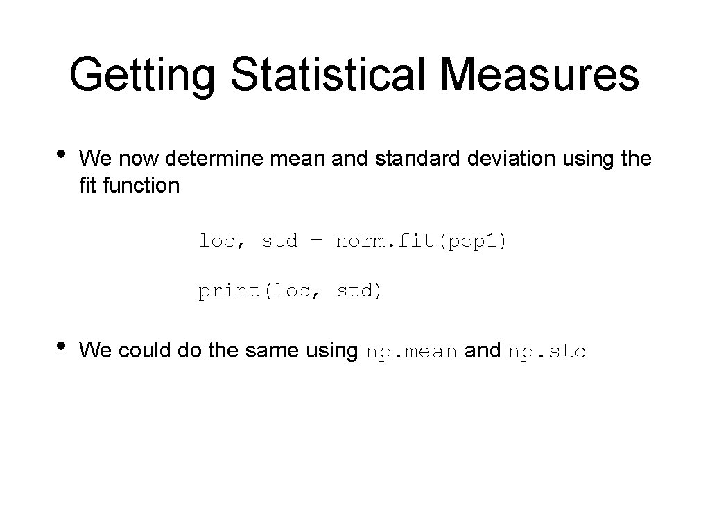
Getting Statistical Measures • We now determine mean and standard deviation using the fit function loc, std = norm. fit(pop 1) print(loc, std) • We could do the same using np. mean and np. std

Getting Statistical Measures • We now create a normal distribution object with this mean and this standard deviation pdf = norm(loc, std). pdf

Getting Statistical Measures • Now, we draw both the histogram and the pdf • The pdf has an integral of 1, so we multiply with the number of elements in the population plt. figure() plt. bar(binscenter, dt, width = bins[1]-bins[0]) plt. plot(binscenter, len(pop 1)*pdf(binscenter), 'red') plt. show()

Getting Statistical Measures

Statistical Tests

Statistical Tests • Statistical test calculates a value — the test statistics — from a sample in order to refute or confirm a hypothesis • Formulate a null hypothesis • This is usually the boring stuff: two samples from the same distribution, mean is where it is expected to be, … • Calculate the probability that the observed statistics or a more significant result has occurred given the null hypothesis • If the probability is small: reject the null hypothesis

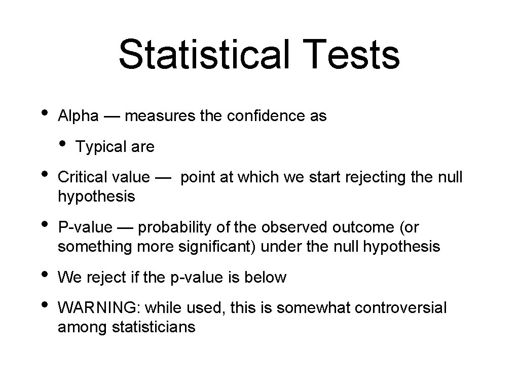
Statistical Tests • Alpha — measures the confidence as • Typical are • Critical value — point at which we start rejecting the null hypothesis • P-value — probability of the observed outcome (or something more significant) under the null hypothesis • • We reject if the p-value is below WARNING: while used, this is somewhat controversial among statisticians

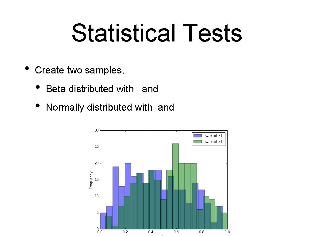
Statistical Tests • Create two samples, • • Beta distributed with and Normally distributed with and

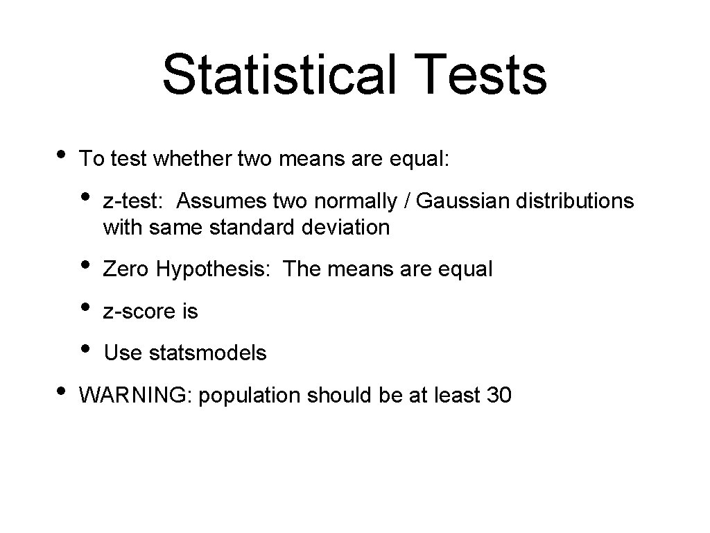
Statistical Tests • • To test whether two means are equal: • z-test: Assumes two normally / Gaussian distributions with same standard deviation • • • Zero Hypothesis: The means are equal z-score is Use statsmodels WARNING: population should be at least 30

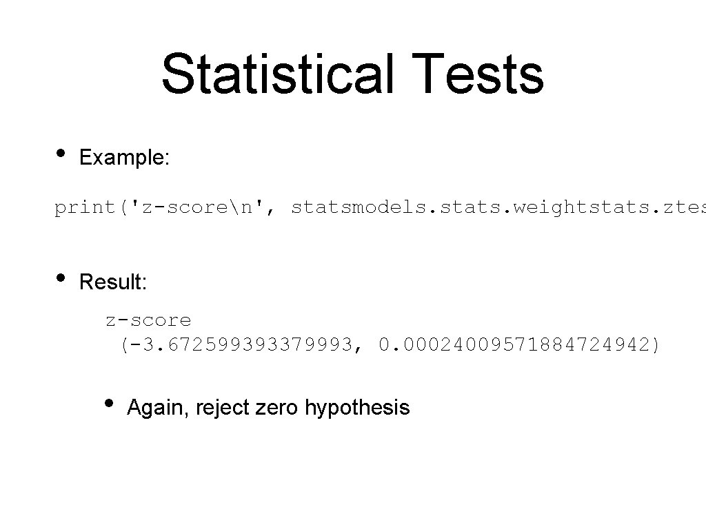
Statistical Tests • Example: print('z-scoren', statsmodels. stats. weightstats. ztes • Result: z-score (-3. 672599393379993, 0. 00024009571884724942) • Again, reject zero hypothesis

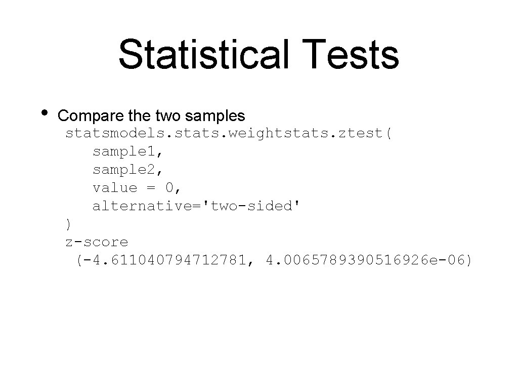
Statistical Tests • Compare the two samples statsmodels. stats. weightstats. ztest( sample 1, sample 2, value = 0, alternative='two-sided' ) z-score (-4. 611040794712781, 4. 0065789390516926 e-06)

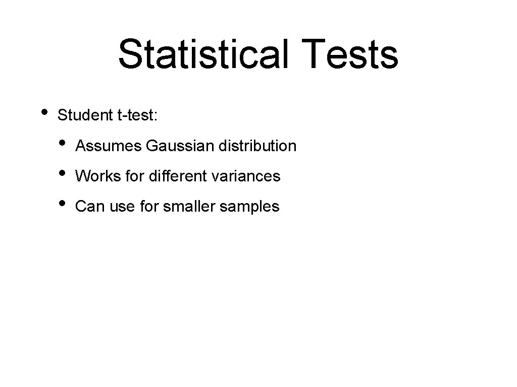
Statistical Tests • Student t-test: • • • Assumes Gaussian distribution Works for different variances Can use for smaller samples

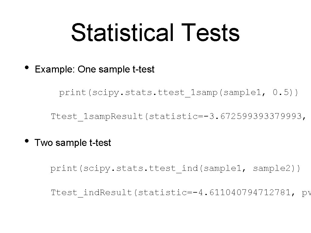
Statistical Tests • Example: One sample t-test print(scipy. stats. ttest_1 samp(sample 1, 0. 5)) Ttest_1 samp. Result(statistic=-3. 672599393379993, • Two sample t-test print(scipy. stats. ttest_ind(sample 1, sample 2)) Ttest_ind. Result(statistic=-4. 611040794712781, pv

Statistical Tests • This is just a sample of important tests

Contingency Tables

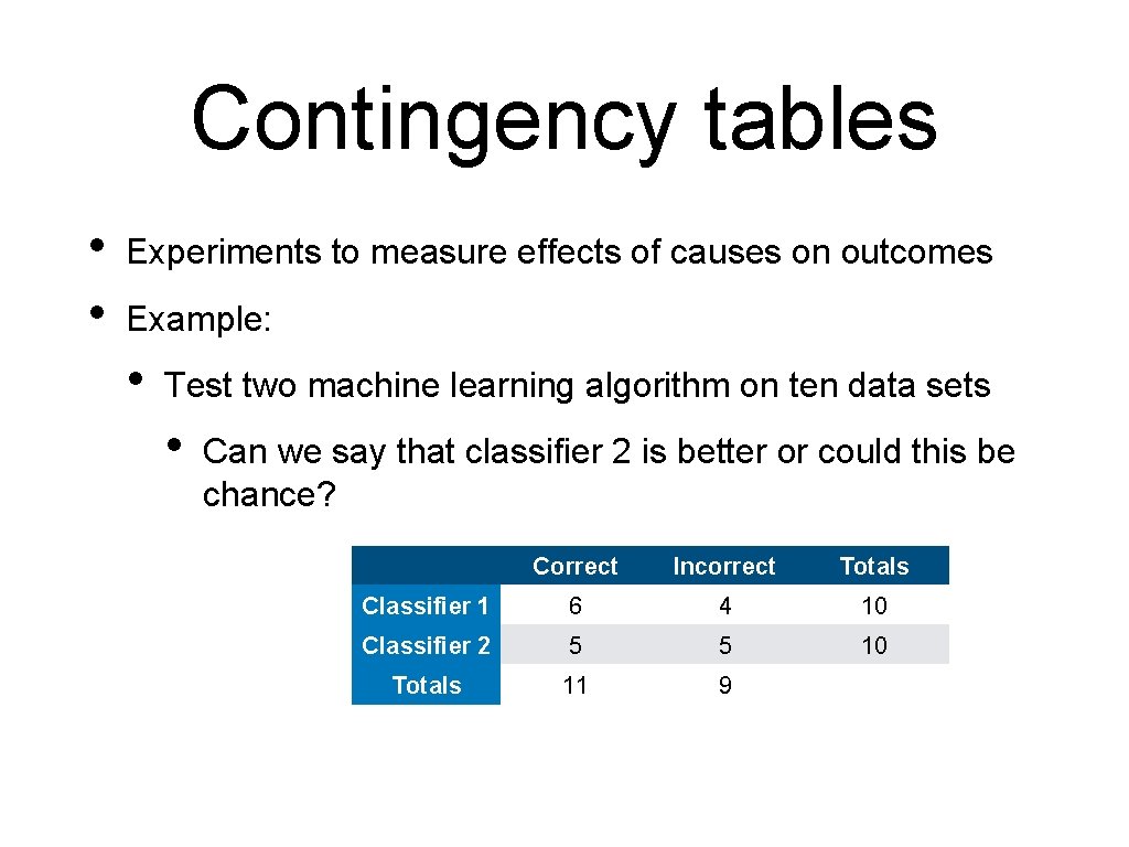
Contingency tables • • Experiments to measure effects of causes on outcomes Example: • Test two machine learning algorithm on ten data sets • Can we say that classifier 2 is better or could this be chance? Correct Incorrect Totals Classifier 1 6 4 10 Classifier 2 5 5 10 Totals 11 9

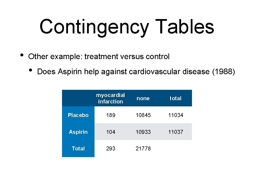
Contingency Tables • Other example: treatment versus control • Does Aspirin help against cardiovascular disease (1988) myocardial infarction none total Placebo 189 10845 11034 Aspirin 104 10933 11037 Total 293 21778

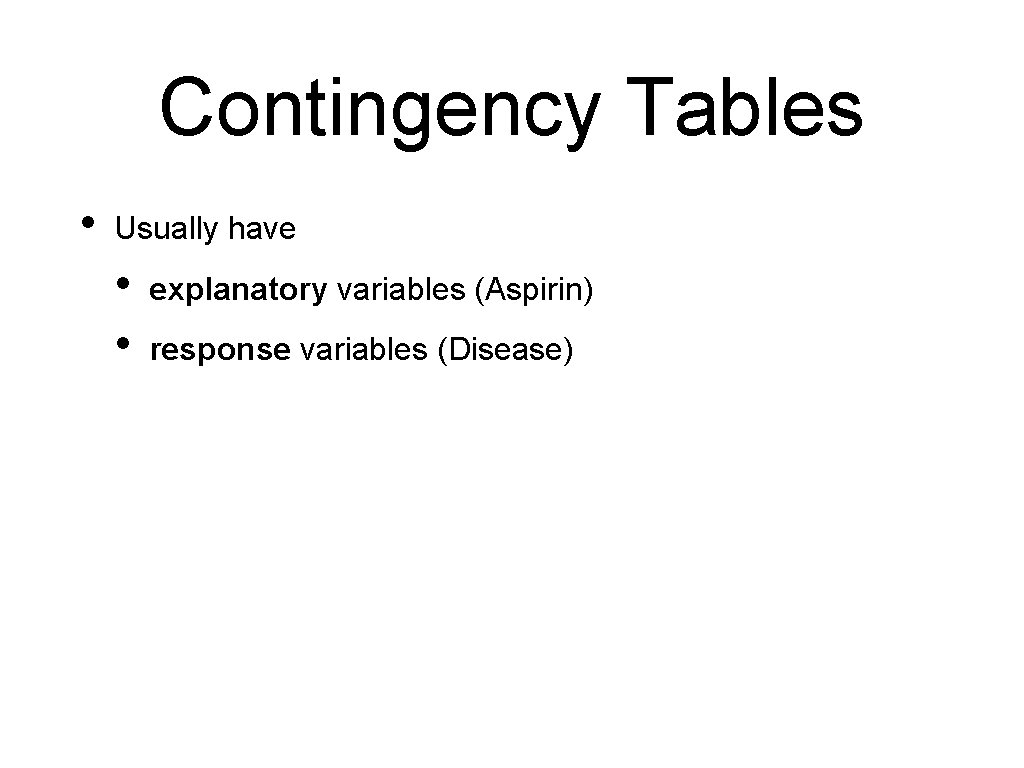
Contingency Tables • Usually have • • explanatory variables (Aspirin) response variables (Disease)

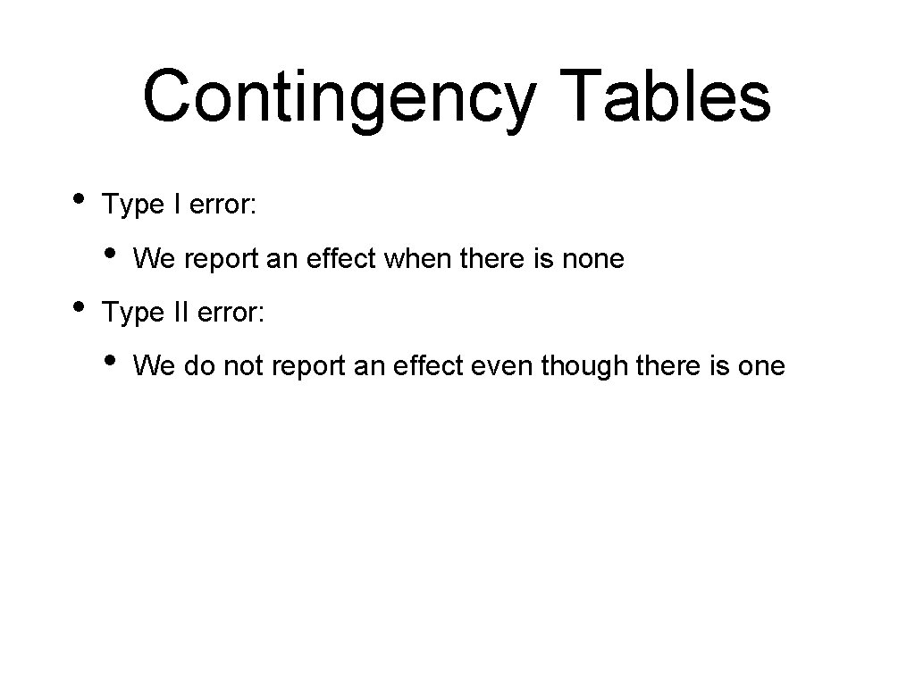
Contingency Tables • Type I error: • • We report an effect when there is none Type II error: • We do not report an effect even though there is one

Contingency Tables • There are many possible statistics • More, if the number of observations is high

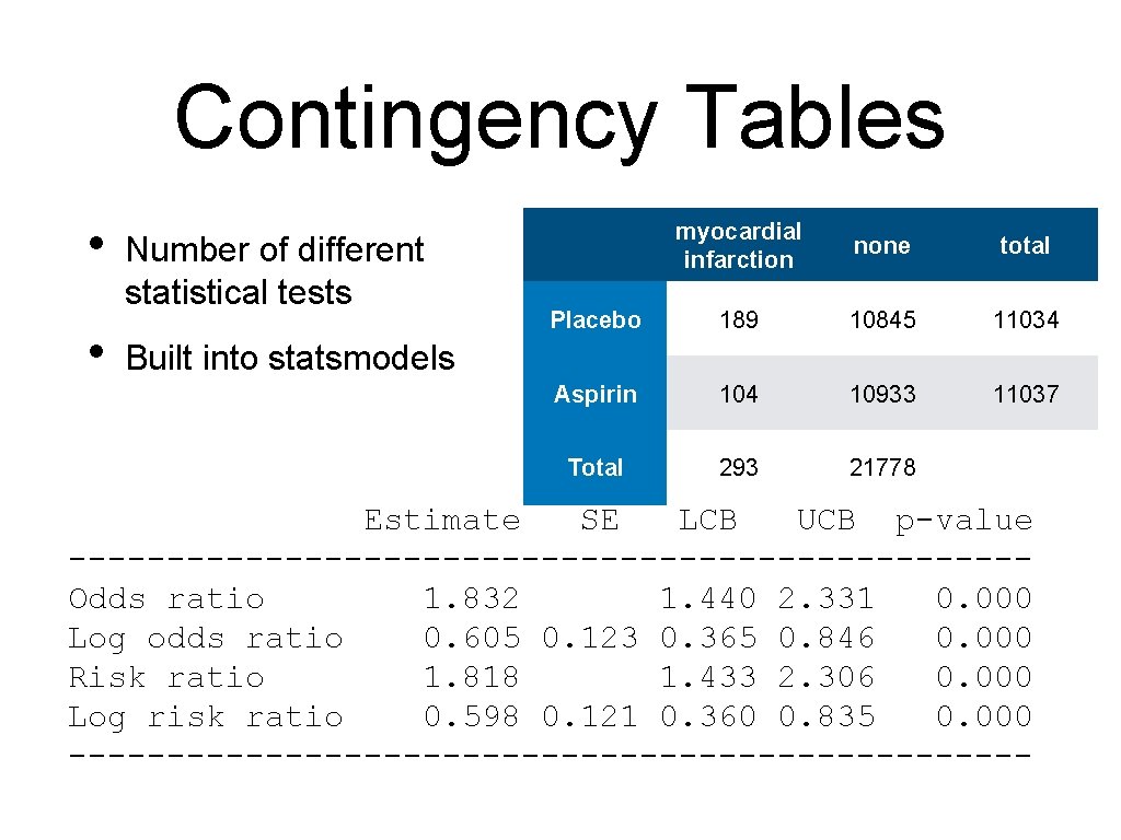
Contingency Tables • • Number of different statistical tests myocardial infarction none total Placebo 189 10845 11034 Aspirin 104 10933 11037 Total 293 21778 Built into statsmodels Estimate SE LCB UCB p-value ------------------------Odds ratio 1. 832 1. 440 2. 331 0. 000 Log odds ratio 0. 605 0. 123 0. 365 0. 846 0. 000 Risk ratio 1. 818 1. 433 2. 306 0. 000 Log risk ratio 0. 598 0. 121 0. 360 0. 835 0. 000 -------------------------

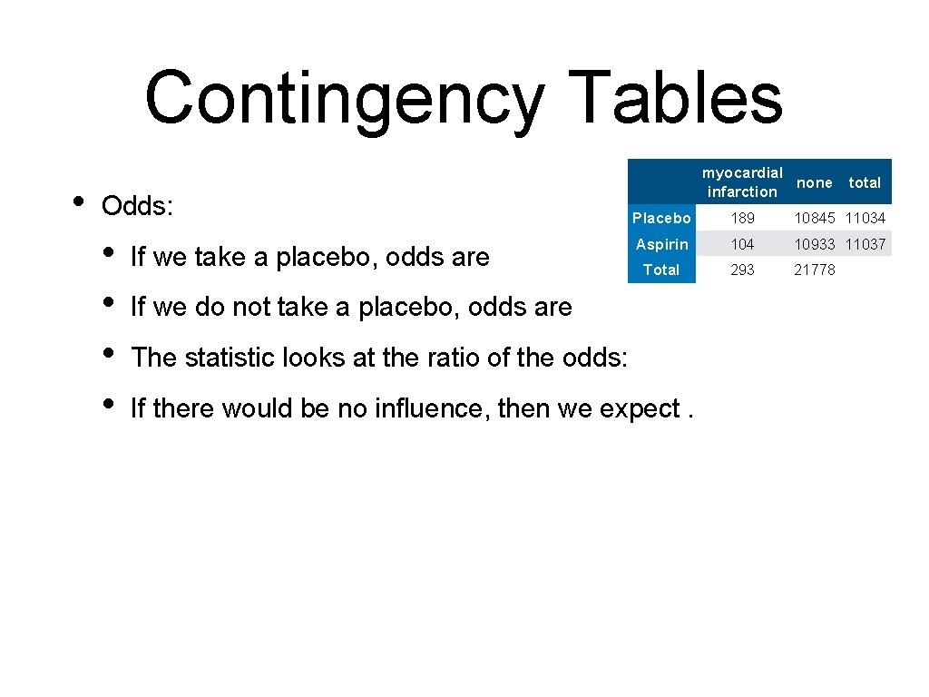
Contingency Tables • Odds: • • If we take a placebo, odds are myocardial none infarction total Placebo 189 10845 11034 Aspirin 104 10933 11037 Total 293 21778 If we do not take a placebo, odds are The statistic looks at the ratio of the odds: If there would be no influence, then we expect.

Contingency Tables • Log odds • • The statistics for odds are heavily skewed Easier to use which can be approximated with a normal distribution

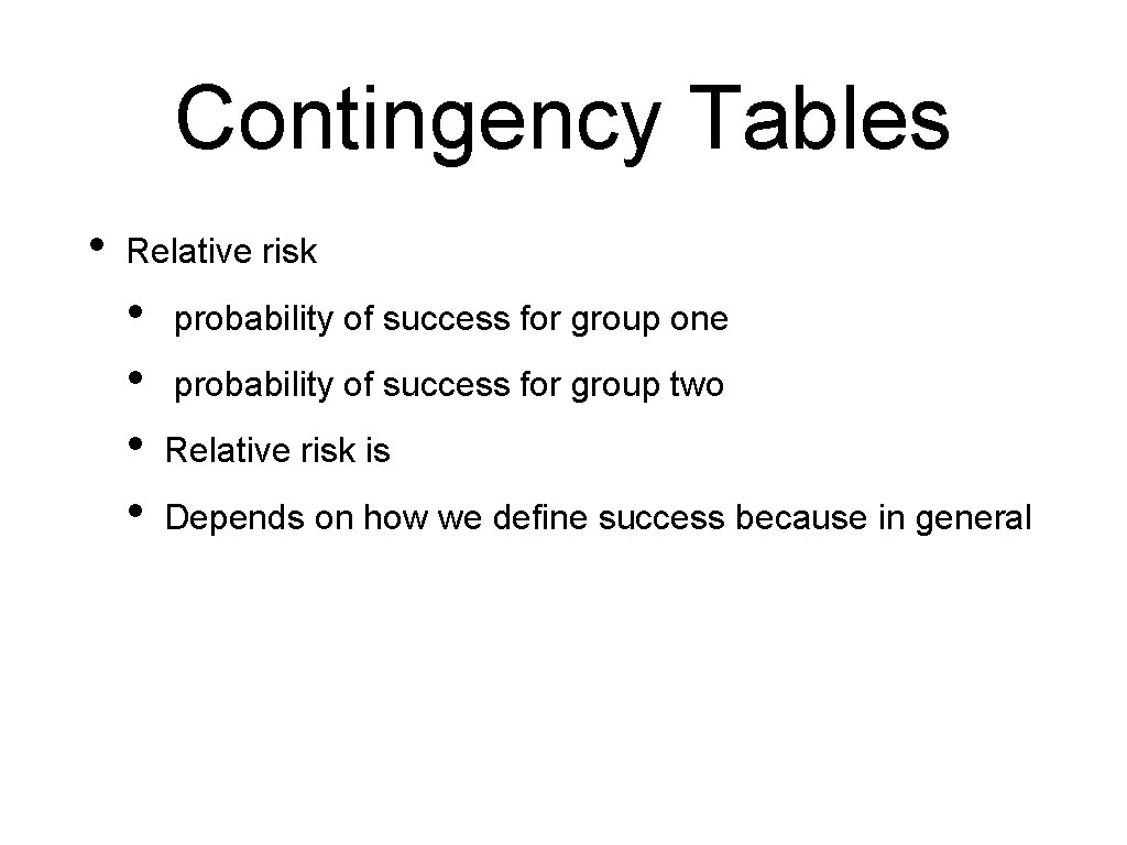
Contingency Tables • Relative risk • • probability of success for group one probability of success for group two Relative risk is Depends on how we define success because in general

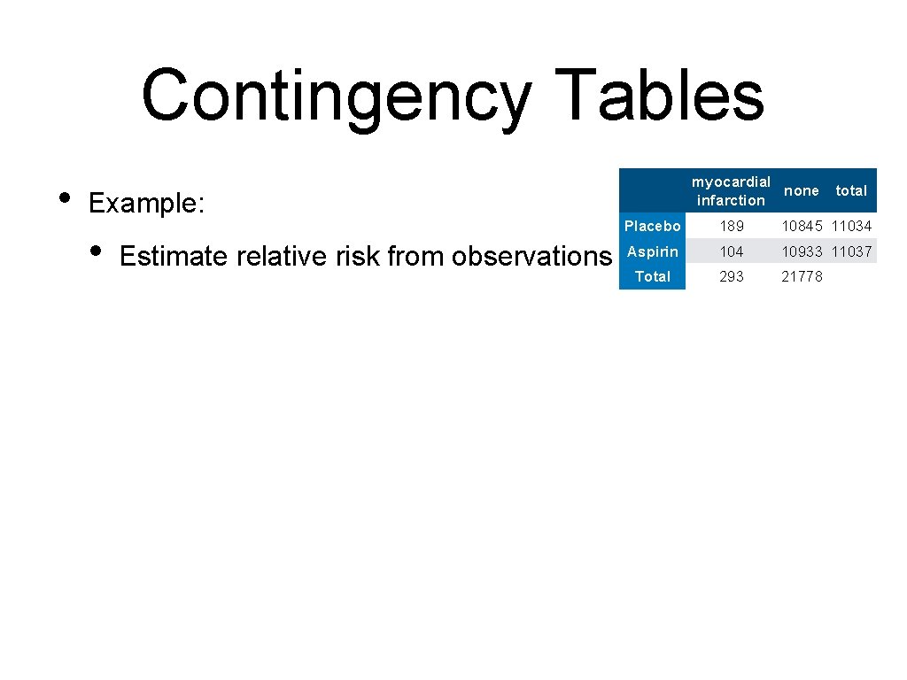
Contingency Tables • Example: • Estimate relative risk from observations myocardial none infarction total Placebo 189 10845 11034 Aspirin 104 10933 11037 Total 293 21778

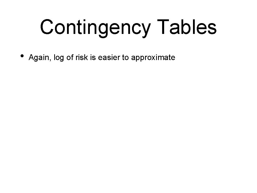
Contingency Tables • Again, log of risk is easier to approximate

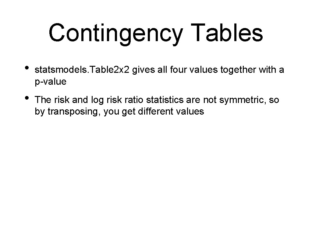
Contingency Tables • statsmodels. Table 2 x 2 gives all four values together with a p-value • The risk and log risk ratio statistics are not symmetric, so by transposing, you get different values

Contingency Tables • • For small samples, we should use Fisher's exact test • If there is no influence of the explanatory variables, then the numbers in the cells are distributed according to a hyper-geometric distribution • With Python, we can apply this even to larger samples Use fisher_exact in scipy. stats

Contingency Tables • Calling Fisher's exact method scipy. stats. fisher_exact(table)) • Output is value of the statistics and the p-value (1. 8320539419087136, 5. 032835599791868 e-07) • Again, we conclude that the difference between Aspirin and Placebo are unlikely to have happened by chance

Testing for Normality

Normality Tests • A large number of models assume that data is or close to normally distributed • If data comes from normal distribution: • • Lots of statistical tricks available If data comes from another distribution: • Maybe use "non-parametic" methods • Use tests to determine whether a given set of data is likely to come from a normal distribution • Step 1: • Use a histogram or scatter-plot of the data

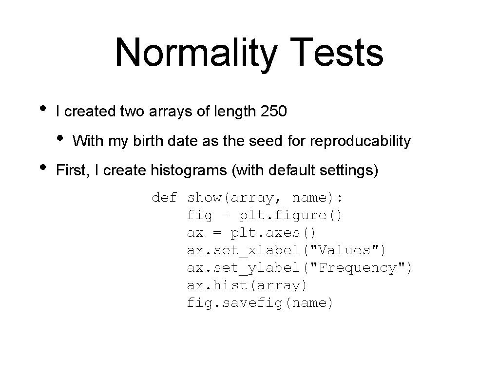
Normality Tests • I created two arrays of length 250 • • With my birth date as the seed for reproducability First, I create histograms (with default settings) def show(array, name): fig = plt. figure() ax = plt. axes() ax. set_xlabel("Values") ax. set_ylabel("Frequency") ax. hist(array) fig. savefig(name)

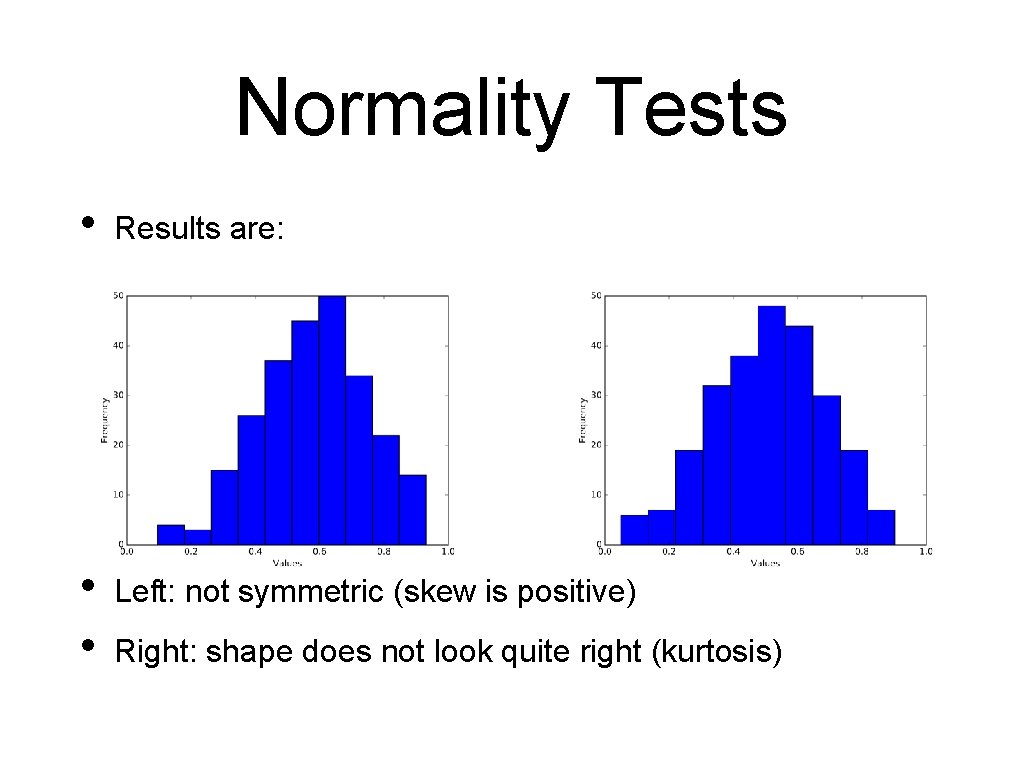
Normality Tests • Results are: • • Left: not symmetric (skew is positive) Right: shape does not look quite right (kurtosis)

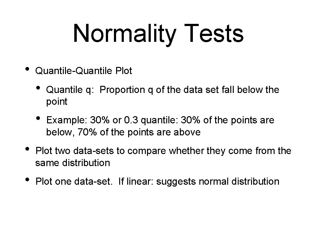
Normality Tests • Quantile-Quantile Plot • Quantile q: Proportion q of the data set fall below the point • Example: 30% or 0. 3 quantile: 30% of the points are below, 70% of the points are above • Plot two data-sets to compare whether they come from the same distribution • Plot one data-set. If linear: suggests normal distribution

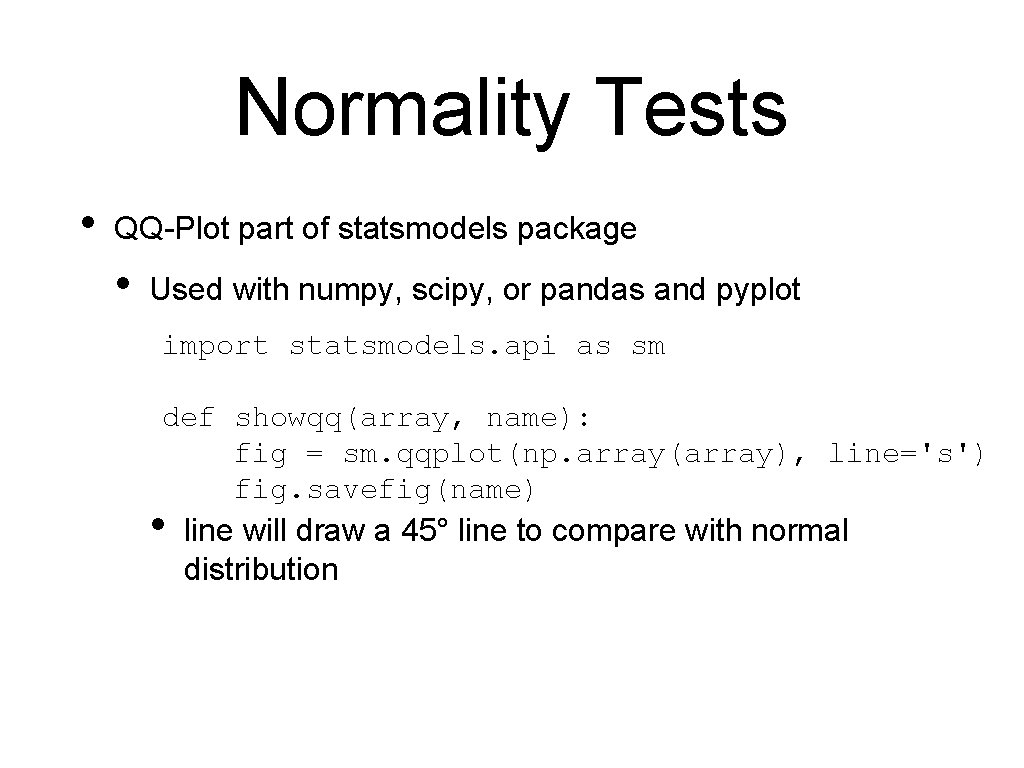
Normality Tests • QQ-Plot part of statsmodels package • Used with numpy, scipy, or pandas and pyplot import statsmodels. api as sm def showqq(array, name): fig = sm. qqplot(np. array(array), line='s') fig. savefig(name) • line will draw a 45° line to compare with normal distribution

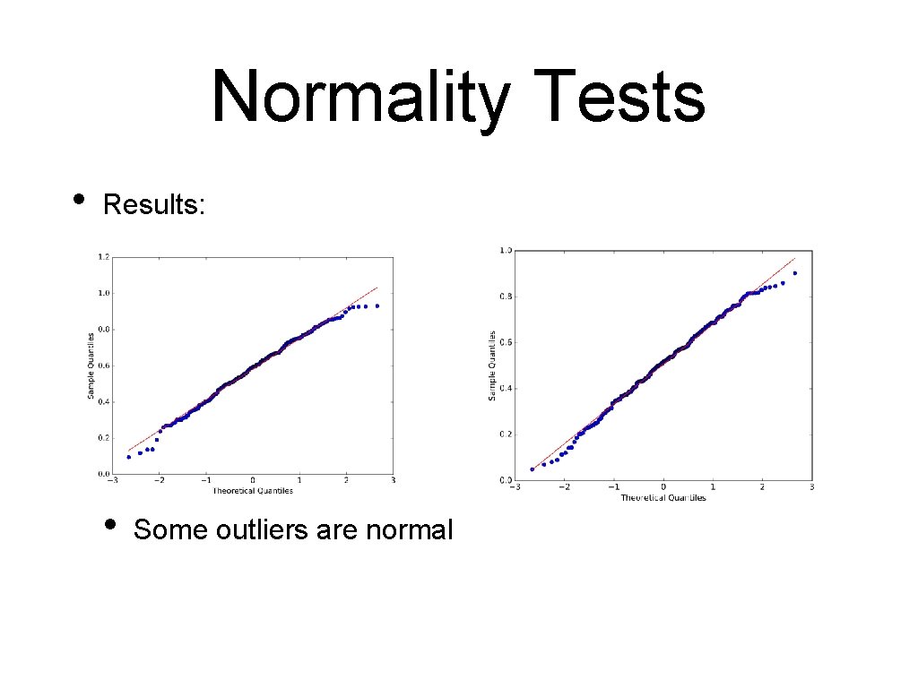
Normality Tests • Results: • Some outliers are normal

Normality Tests • Statistical tests: • • Takes data and calculates a test statistics • Calculates the probability of the test value assuming that a null hypothesis is true • If the probability is too small, concludes that the null hypothesis is false In Scipy: • • • Null hypothesis: "Distribution is normal" Returns a p-value If p-value is smaller than : reject the Null Hypothesis, otherwise see it supported by data

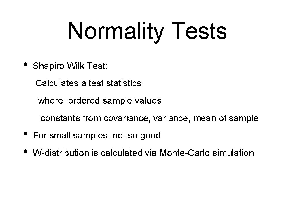
Normality Tests • Shapiro Wilk Test: Calculates a test statistics where ordered sample values constants from covariance, mean of sample • • For small samples, not so good W-distribution is calculated via Monte-Carlo simulation

Normality Tests • Use scipy. stats. shapiro • • Input is the data Output is the W-value and the p-value import scipy. stats def getshapiro(array): return scipy. stats. shapiro(array)

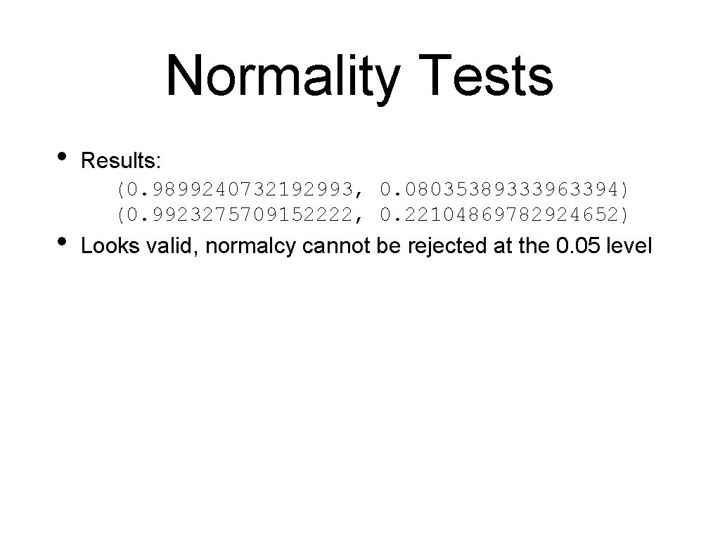
Normality Tests • • Results: (0. 9899240732192993, 0. 08035389333963394) (0. 9923275709152222, 0. 22104869782924652) Looks valid, normalcy cannot be rejected at the 0. 05 level

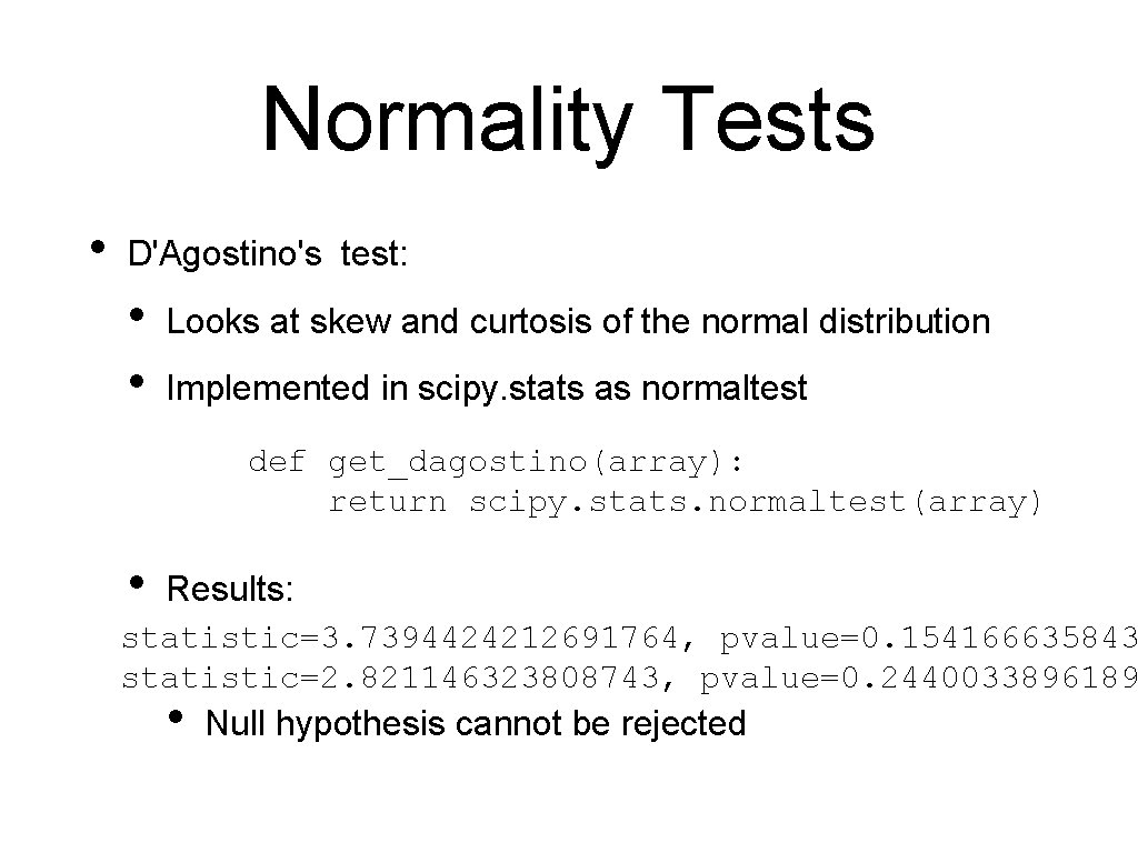
Normality Tests • D'Agostino's test: • • Looks at skew and curtosis of the normal distribution Implemented in scipy. stats as normaltest def get_dagostino(array): return scipy. stats. normaltest(array) • Results: statistic=3. 7394424212691764, pvalue=0. 154166635843 statistic=2. 821146323808743, pvalue=0. 2440033896189 • Null hypothesis cannot be rejected

Normality Tests • Anderson Darling • Comes from the Kolmogorov Smirnov test • KS tests for the distance between the cumulative probability of two samples or one sample with a reference distribution

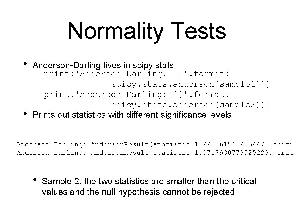
Normality Tests • • Anderson-Darling lives in scipy. stats print('Anderson Darling: {}'. format( scipy. stats. anderson(sample 1))) print('Anderson Darling: {}'. format( scipy. stats. anderson(sample 2))) Prints out statistics with different significance levels Anderson Darling: Anderson. Result(statistic=1. 998061561955467, critic Anderson Darling: Anderson. Result(statistic=1. 0717930773325293, criti • Sample 2: the two statistics are smaller than the critical values and the null hypothesis cannot be rejected

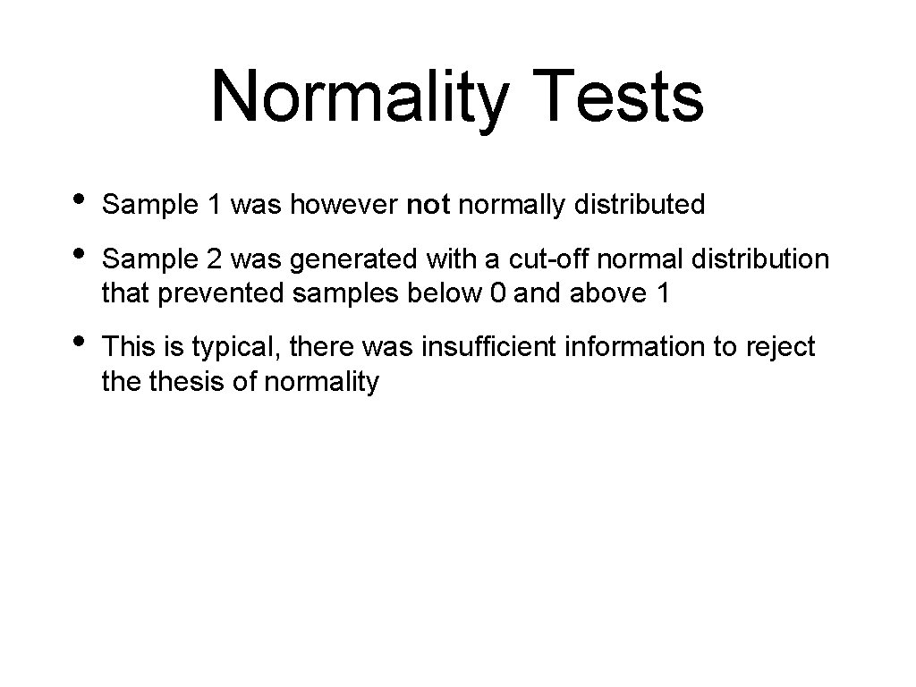
Normality Tests • • Sample 1 was however not normally distributed • This is typical, there was insufficient information to reject thesis of normality Sample 2 was generated with a cut-off normal distribution that prevented samples below 0 and above 1

Limitations

Limitations • With a p value of 0. 05, one in twenty tests is likely to give us a false positive • Rate of false negatives is also around that

Limitations • Not being able to reject the zero hypothesis does not mean that the hypothesis is wrong

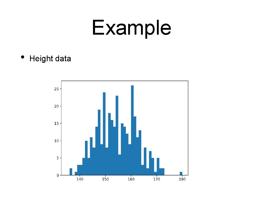
Example • Height data

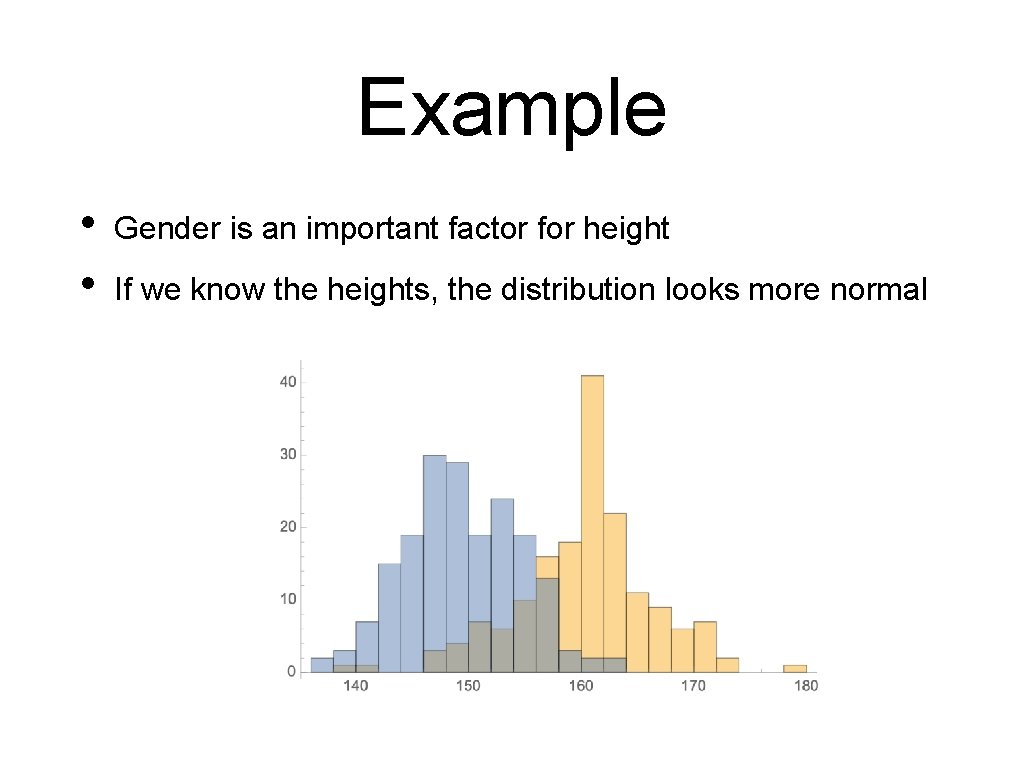
Example • • Gender is an important factor for height If we know the heights, the distribution looks more normal

Example • When we apply normality tests: • • • Female is normally distributed Male is not normally distributed according to Anderson Complete population is normally distributed

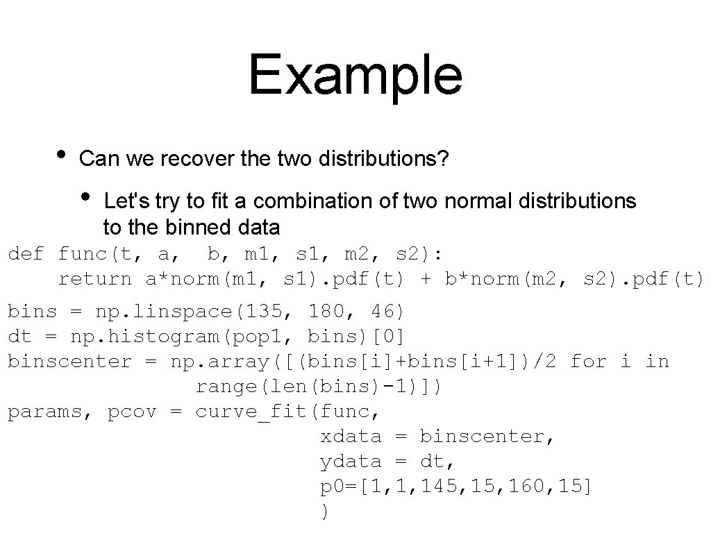
Example • Can we recover the two distributions? • Let's try to fit a combination of two normal distributions to the binned data def func(t, a, b, m 1, s 1, m 2, s 2): return a*norm(m 1, s 1). pdf(t) + b*norm(m 2, s 2). pdf(t) bins = np. linspace(135, 180, 46) dt = np. histogram(pop 1, bins)[0] binscenter = np. array([(bins[i]+bins[i+1])/2 for i in range(len(bins)-1)]) params, pcov = curve_fit(func, xdata = binscenter, ydata = dt, p 0=[1, 1, 145, 160, 15] )

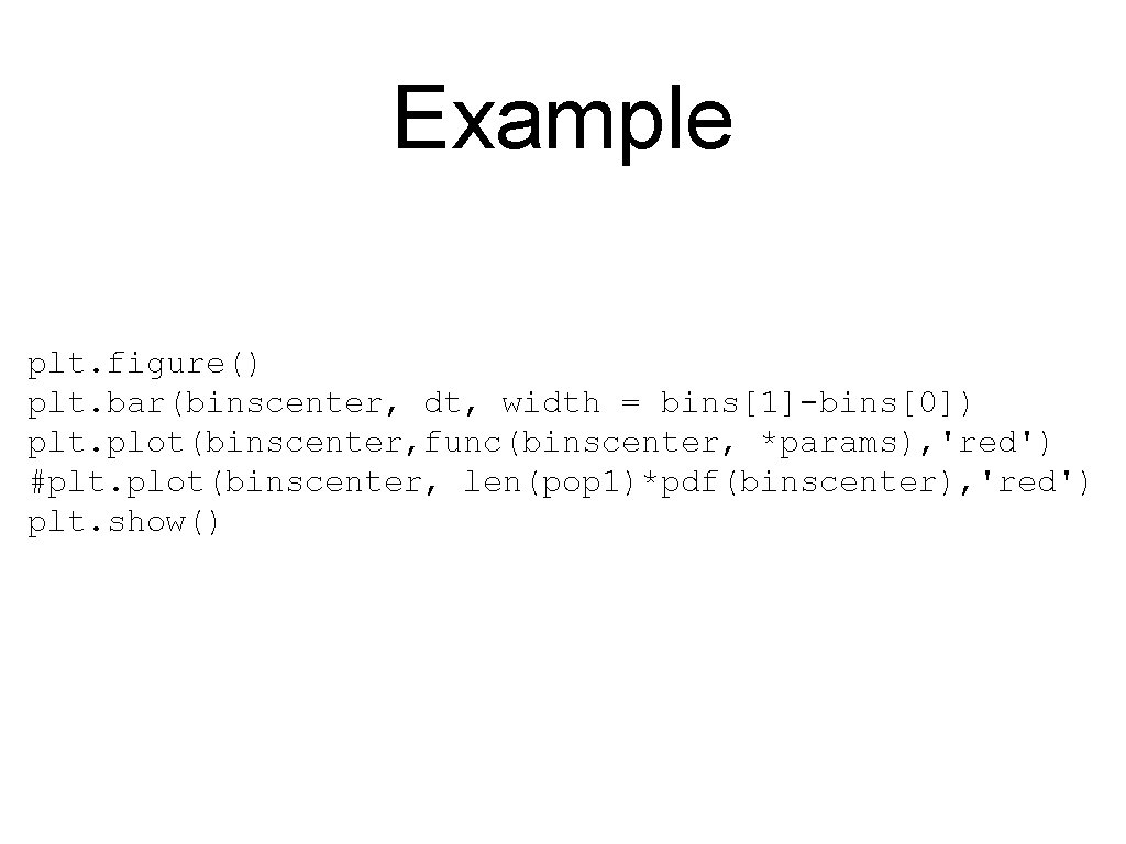
Example plt. figure() plt. bar(binscenter, dt, width = bins[1]-bins[0]) plt. plot(binscenter, func(binscenter, *params), 'red') #plt. plot(binscenter, len(pop 1)*pdf(binscenter), 'red') plt. show()

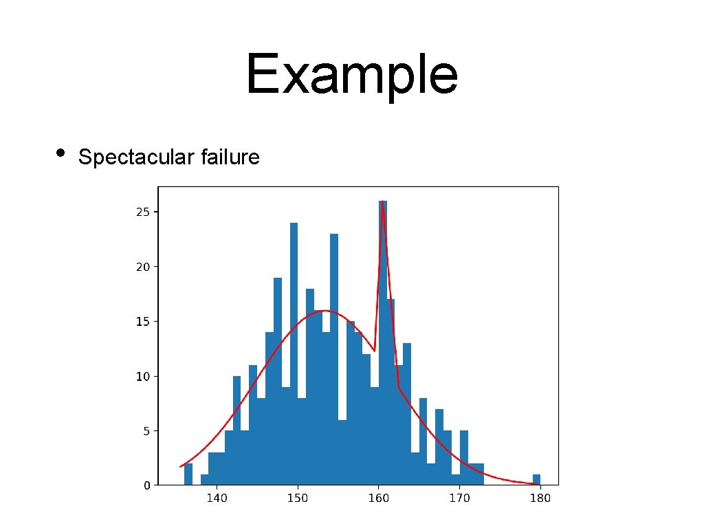
Example • Spectacular failure

Conclusions • Numpy has a very broad selection of random number generators • Scipy. stats has a very good set of implementations for many standard statistical tests • Which cannot overcome limitations in the data

Readings • Scipy Lecture notes p. 195 ff