STATS 330 Lecture 12 11272020 330 lecture 12

STATS 330: Lecture 12 11/27/2020 330 lecture 12 1

Diagnostics 4 Aim of today’s lecture To discuss diagnostics for independence 11/27/2020 330 lecture 12 2

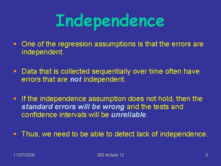
Independence § One of the regression assumptions is that the errors are independent. § Data that is collected sequentially over time often have errors that are not independent. § If the independence assumption does not hold, then the standard errors will be wrong and the tests and confidence intervals will be unreliable. § Thus, we need to be able to detect lack of independence. 11/27/2020 330 lecture 12 3

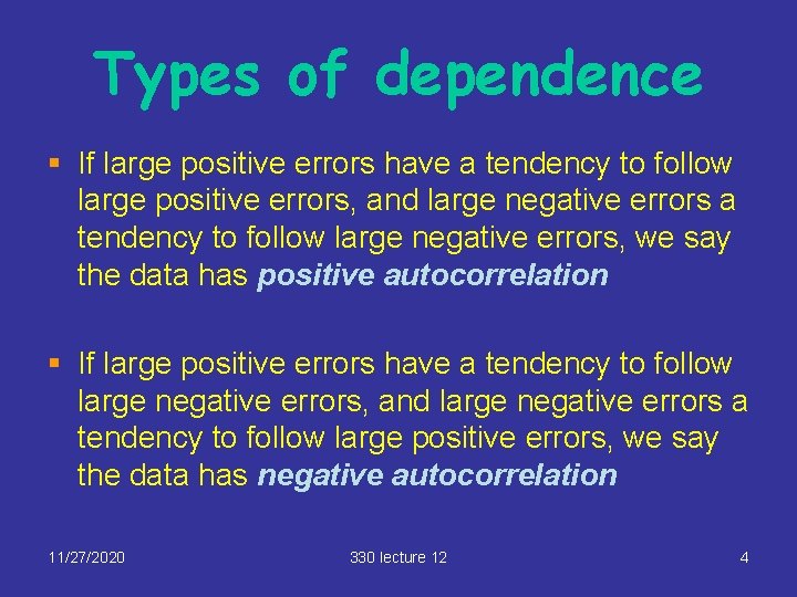
Types of dependence § If large positive errors have a tendency to follow large positive errors, and large negative errors a tendency to follow large negative errors, we say the data has positive autocorrelation § If large positive errors have a tendency to follow large negative errors, and large negative errors a tendency to follow large positive errors, we say the data has negative autocorrelation 11/27/2020 330 lecture 12 4

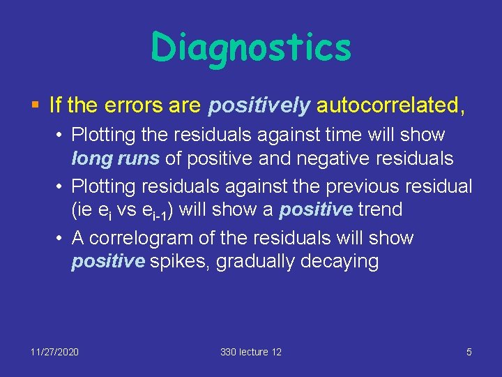
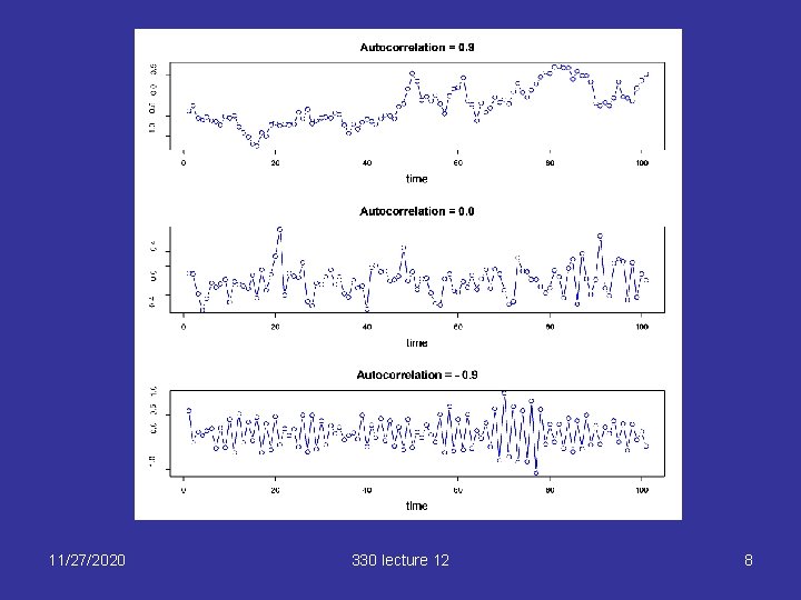
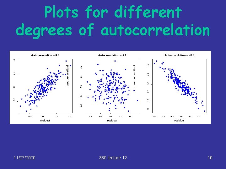
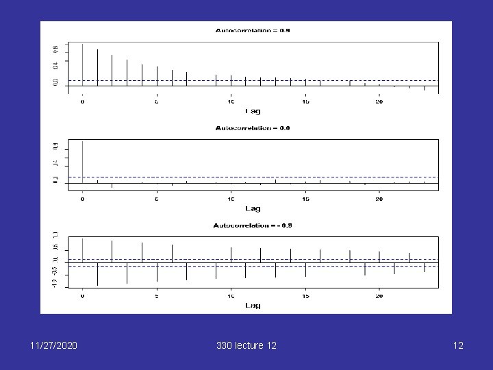
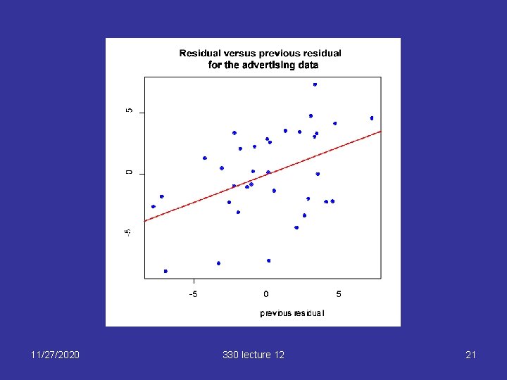
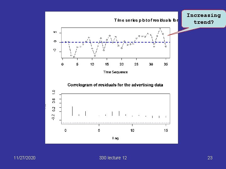
Diagnostics § If the errors are positively autocorrelated, • Plotting the residuals against time will show long runs of positive and negative residuals • Plotting residuals against the previous residual (ie ei vs ei-1) will show a positive trend • A correlogram of the residuals will show positive spikes, gradually decaying 11/27/2020 330 lecture 12 5

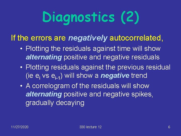
Diagnostics (2) If the errors are negatively autocorrelated, • Plotting the residuals against time will show alternating positive and negative residuals • Plotting residuals against the previous residual (ie ei vs ei-1) will show a negative trend • A correlogram of the residuals will show alternating positive and negative spikes, gradually decaying 11/27/2020 330 lecture 12 6

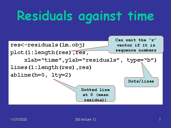
Residuals against time Can omit the “x” vector if it is sequence numbers res<-residuals(lm. obj) plot(1: length(res), res, xlab=“time”, ylab=“residuals”, type=“b”) lines(1: length(res), res) abline(h=0, lty=2) Dots/lines Dotted line at 0 (mean residual) 11/27/2020 330 lecture 12 7

11/27/2020 330 lecture 12 8

Residuals against previous res<-residuals(lm. obj) n<-length(res) plot. res<-res[-1] # element 1 has no previous prev. res<-res[-n] # have to be equal length plot(prev. res, plot. res, xlab=“previous residual”, ylab=“residual”) 11/27/2020 330 lecture 12 9

Plots for different degrees of autocorrelation 11/27/2020 330 lecture 12 10

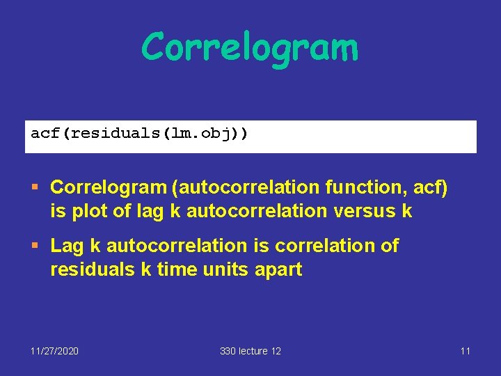
Correlogram acf(residuals(lm. obj)) § Correlogram (autocorrelation function, acf) is plot of lag k autocorrelation versus k § Lag k autocorrelation is correlation of residuals k time units apart 11/27/2020 330 lecture 12 11

11/27/2020 330 lecture 12 12

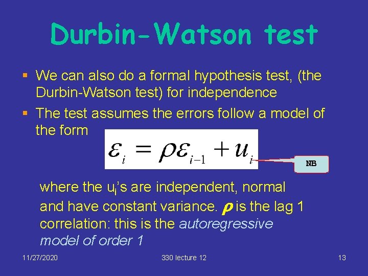
Durbin-Watson test § We can also do a formal hypothesis test, (the Durbin-Watson test) for independence § The test assumes the errors follow a model of the form NB where the ui’s are independent, normal and have constant variance. r is the lag 1 correlation: this is the autoregressive model of order 1 11/27/2020 330 lecture 12 13

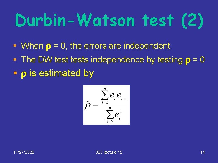
Durbin-Watson test (2) § When r = 0, the errors are independent § The DW tests independence by testing r = 0 § r is estimated by 11/27/2020 330 lecture 12 14

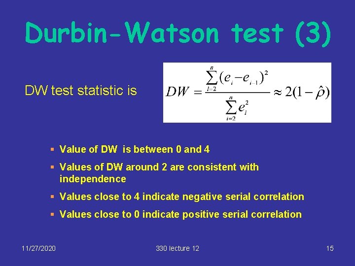
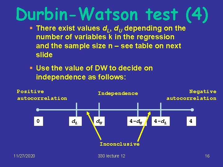
Durbin-Watson test (3) DW test statistic is § Value of DW is between 0 and 4 § Values of DW around 2 are consistent with independence § Values close to 4 indicate negative serial correlation § Values close to 0 indicate positive serial correlation 11/27/2020 330 lecture 12 15

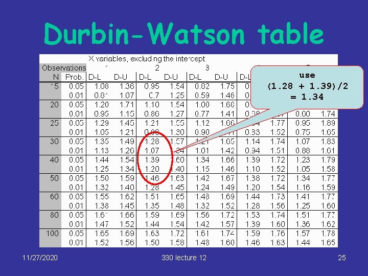
Durbin-Watson test (4) § There exist values d. L, d. U depending on the number of variables k in the regression and the sample size n – see table on next slide § Use the value of DW to decide on independence as follows: Positive autocorrelation 0 Independence d. L d. U 4 -d. U Negative autocorrelation 4 -d. L 4 Inconclusive 11/27/2020 330 lecture 12 16

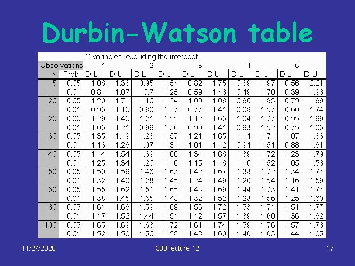
Durbin-Watson table 11/27/2020 330 lecture 12 17

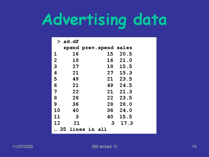
Example: the advertising data § Sales and advertising data § Data on monthly sales and advertising spend for 35 months § Model is Sales ~ spend + prev. spend (prev. spend = spend in previous month) 11/27/2020 330 lecture 12 18

Advertising data > ad. df spend prev. spend sales 1 16 15 20. 5 2 18 16 21. 0 3 27 18 15. 5 4 21 27 15. 3 5 49 21 23. 5 6 21 49 24. 5 7 22 21 21. 3 8 28 22 23. 5 9 36 28 28. 0 10 40 36 24. 0 11 3 40 15. 5 12 21 3 17. 3 … 35 lines in all 11/27/2020 330 lecture 12 19

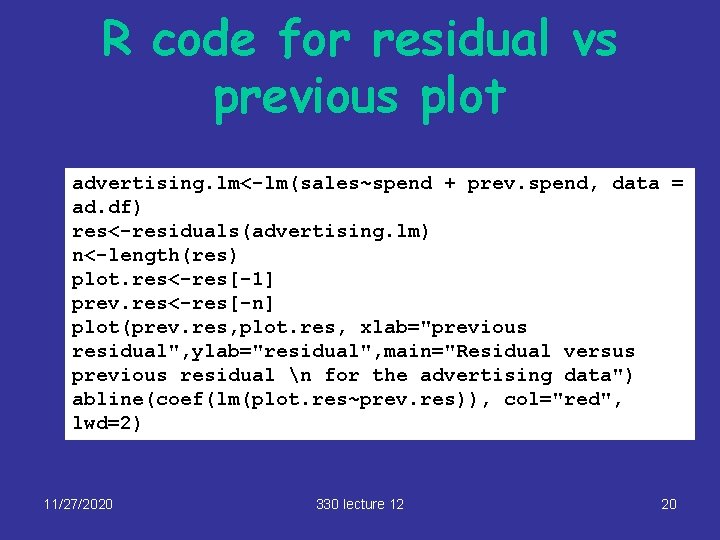
R code for residual vs previous plot advertising. lm<-lm(sales~spend + prev. spend, data = ad. df) res<-residuals(advertising. lm) n<-length(res) plot. res<-res[-1] prev. res<-res[-n] plot(prev. res, plot. res, xlab="previous residual", ylab="residual", main="Residual versus previous residual n for the advertising data") abline(coef(lm(plot. res~prev. res)), col="red", lwd=2) 11/27/2020 330 lecture 12 20

11/27/2020 330 lecture 12 21

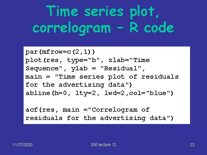
Time series plot, correlogram – R code par(mfrow=c(2, 1)) plot(res, type="b", xlab="Time Sequence", ylab = "Residual", main = "Time series plot of residuals for the advertising data") abline(h=0, lty=2, lwd=2, col="blue") acf(res, main ="Correlogram of residuals for the advertising data") 11/27/2020 330 lecture 12 22

Increasing trend? 11/27/2020 330 lecture 12 23

Calculating DW > rhohat<-cor(plot. res, prev. res) > rhohat [1] 0. 4450734 > DW<-2*(1 -rhohat) > DW [1] 1. 109853 For n=35 and k=2, d. L = 1. 34. Since DW = 1. 109 < d. L = 1. 34 , strong evidence of positive serial correlation 11/27/2020 330 lecture 12 24

Durbin-Watson table use (1. 28 + 1. 39)/2 = 1. 34 11/27/2020 330 lecture 12 25

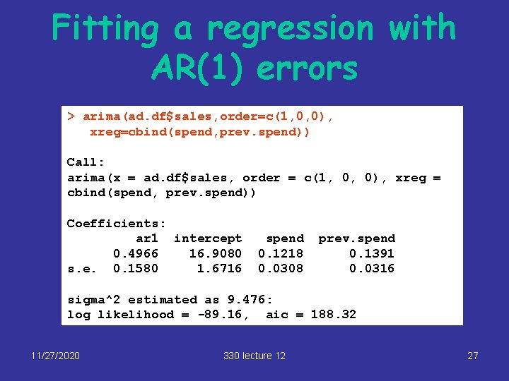
Remedy (1) § If we detect serial correlation, we need to fit special time series models to the data. § For full details see STATS 326/726. § Assuming that the AR(1) model is ok, we can use the arima function in R to fit the regression 11/27/2020 330 lecture 12 26

Fitting a regression with AR(1) errors > arima(ad. df$sales, order=c(1, 0, 0), xreg=cbind(spend, prev. spend)) Call: arima(x = ad. df$sales, order = c(1, 0, 0), xreg = cbind(spend, prev. spend)) Coefficients: ar 1 intercept 0. 4966 16. 9080 s. e. 0. 1580 1. 6716 spend 0. 1218 0. 0308 prev. spend 0. 1391 0. 0316 sigma^2 estimated as 9. 476: log likelihood = -89. 16, aic = 188. 32 11/27/2020 330 lecture 12 27

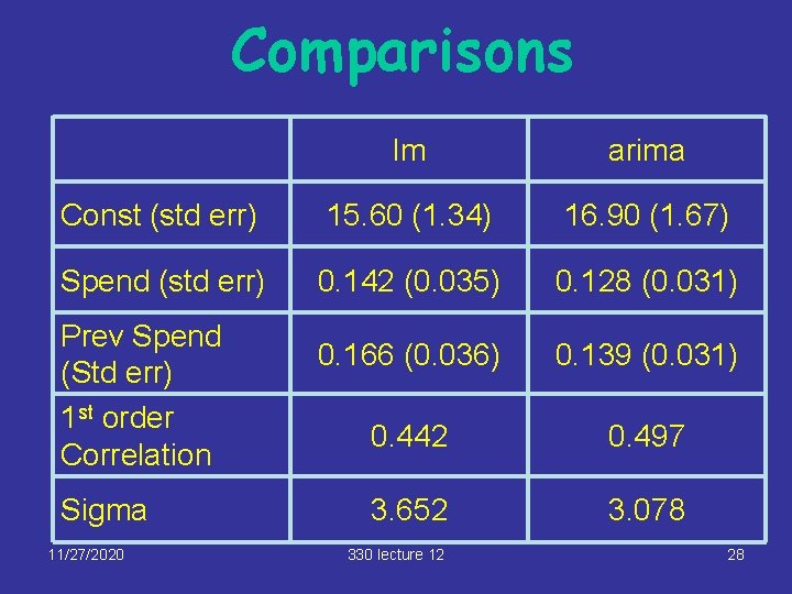
Comparisons lm arima Const (std err) 15. 60 (1. 34) 16. 90 (1. 67) Spend (std err) 0. 142 (0. 035) 0. 128 (0. 031) 0. 166 (0. 036) 0. 139 (0. 031) 0. 442 0. 497 3. 652 3. 078 Prev Spend (Std err) 1 st order Correlation Sigma 11/27/2020 330 lecture 12 28

Remedy (2) § Recall there was a trend in the time series plot of the residuals, these seem related to time § Thus, time is a “lurking variable” , a variable that should be in the regression but isn’t § Try model Sales ~ spend + prev. spend + time 11/27/2020 330 lecture 12 29

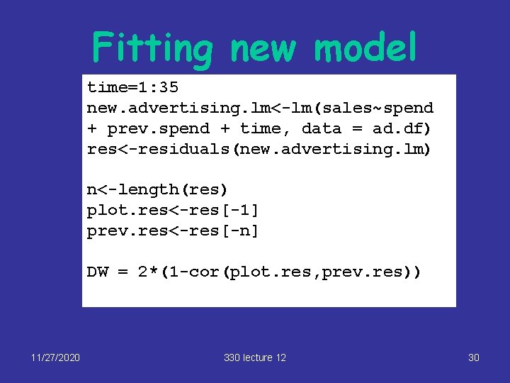
Fitting new model time=1: 35 new. advertising. lm<-lm(sales~spend + prev. spend + time, data = ad. df) res<-residuals(new. advertising. lm) n<-length(res) plot. res<-res[-1] prev. res<-res[-n] DW = 2*(1 -cor(plot. res, prev. res)) 11/27/2020 330 lecture 12 30

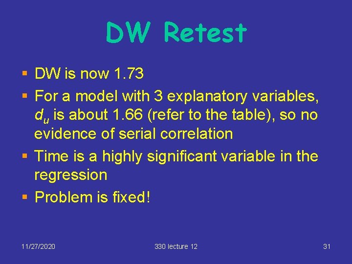
DW Retest § DW is now 1. 73 § For a model with 3 explanatory variables, du is about 1. 66 (refer to the table), so no evidence of serial correlation § Time is a highly significant variable in the regression § Problem is fixed! 11/27/2020 330 lecture 12 31