Stats 330 Lecture 28 Department of Statistics 2012

Stats 330: Lecture 28 © Department of Statistics 2012 STATS 330 Lecture 28: Slide 1

Plan of the day In today’s lecture we apply Poisson regression to the analysis of contingency tables having 3 or 4 dimensions. Topics – Types of independence – Connection between independence and interactions for 3 and 4 dimensional tables – Hierarchical models – Graphical models – Examples Reference: Coursebook, sections 5. 3, 5. 3. 1 © Department of Statistics 2012 STATS 330 Lecture 28: Slide 2

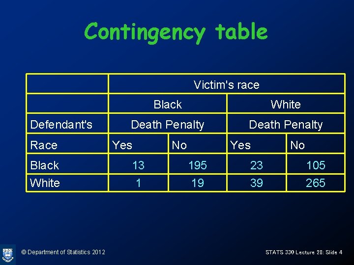
Example: the Florida murder data • 326 convicted murderers in Florida, 19761977 • Classified by – Death penalty (n/y) – Victims race (black/white) – Defendants race (black/white) © Department of Statistics 2012 STATS 330 Lecture 28: Slide 3

Contingency table Victim's race Defendant's Race Black White Death Penalty Yes No Black 13 195 23 105 White 1 19 39 265 © Department of Statistics 2012 STATS 330 Lecture 28: Slide 4

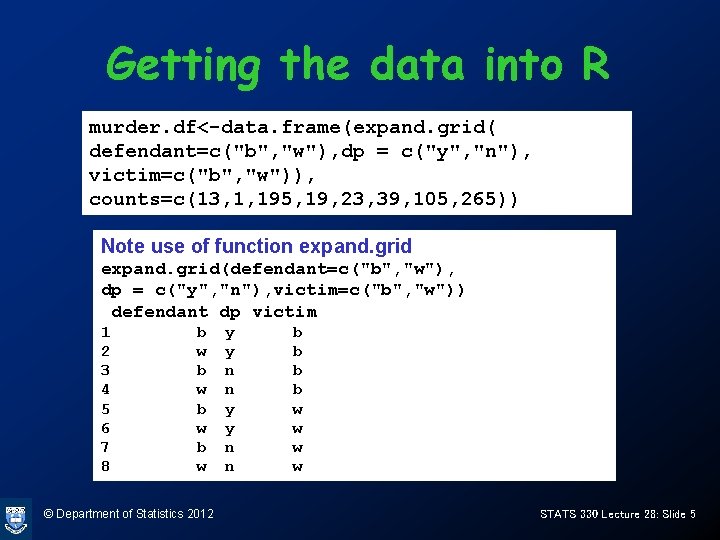
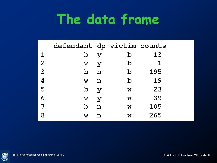
Getting the data into R murder. df<-data. frame(expand. grid( defendant=c("b", "w"), dp = c("y", "n"), victim=c("b", "w")), counts=c(13, 1, 195, 19, 23, 39, 105, 265)) Note use of function expand. grid(defendant=c("b", "w"), dp = c("y", "n"), victim=c("b", "w")) defendant dp victim 1 2 3 4 5 6 7 8 b w b w © Department of Statistics 2012 y y n n b b w w STATS 330 Lecture 28: Slide 5

The data frame 1 2 3 4 5 6 7 8 defendant b w b w © Department of Statistics 2012 dp victim counts y b 13 y b 1 n b 195 n b 19 y w 23 y w 39 n w 105 n w 265 STATS 330 Lecture 28: Slide 6

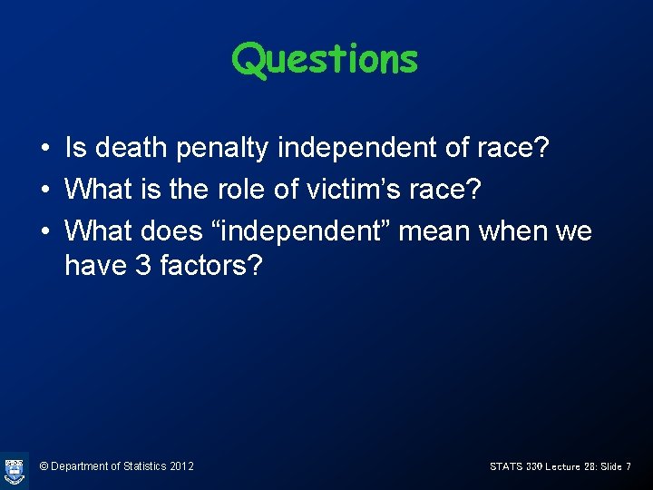
Questions • Is death penalty independent of race? • What is the role of victim’s race? • What does “independent” mean when we have 3 factors? © Department of Statistics 2012 STATS 330 Lecture 28: Slide 7

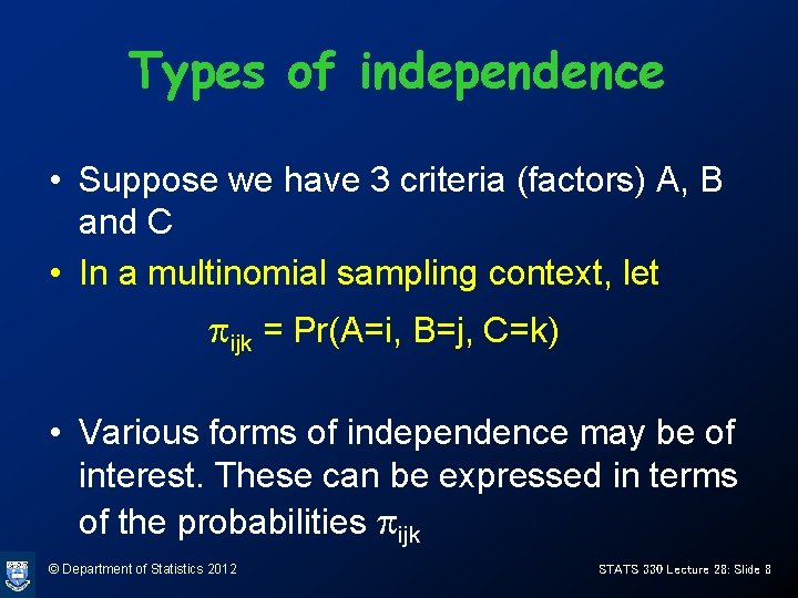
Types of independence • Suppose we have 3 criteria (factors) A, B and C • In a multinomial sampling context, let pijk = Pr(A=i, B=j, C=k) • Various forms of independence may be of interest. These can be expressed in terms of the probabilities pijk © Department of Statistics 2012 STATS 330 Lecture 28: Slide 8

Marginal probabilities © Department of Statistics 2012 STATS 330 Lecture 28: Slide 9

Marginal probabilities (ii) © Department of Statistics 2012 STATS 330 Lecture 28: Slide 10

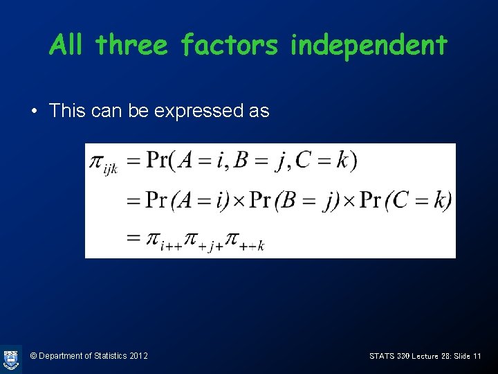
All three factors independent • This can be expressed as © Department of Statistics 2012 STATS 330 Lecture 28: Slide 11

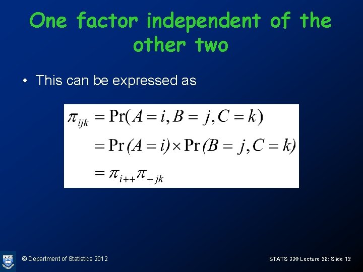
One factor independent of the other two • This can be expressed as © Department of Statistics 2012 STATS 330 Lecture 28: Slide 12

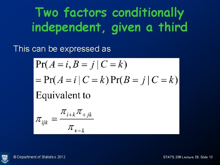
Two factors conditionally independent, given a third This can be expressed as © Department of Statistics 2012 STATS 330 Lecture 28: Slide 13

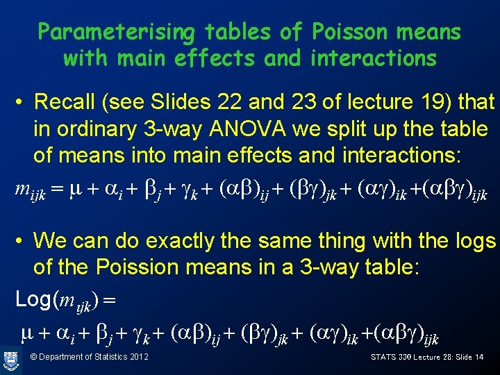
Parameterising tables of Poisson means with main effects and interactions • Recall (see Slides 22 and 23 of lecture 19) that in ordinary 3 -way ANOVA we split up the table of means into main effects and interactions: mijk = m + ai + bj + gk + (ab)ij + (bg)jk + (ag)ik +(abg)ijk • We can do exactly the same thing with the logs of the Poission means in a 3 -way table: Log(mijk) = m + ai + bj + gk + (ab)ij + (bg)jk + (ag)ik +(abg)ijk © Department of Statistics 2012 STATS 330 Lecture 28: Slide 14

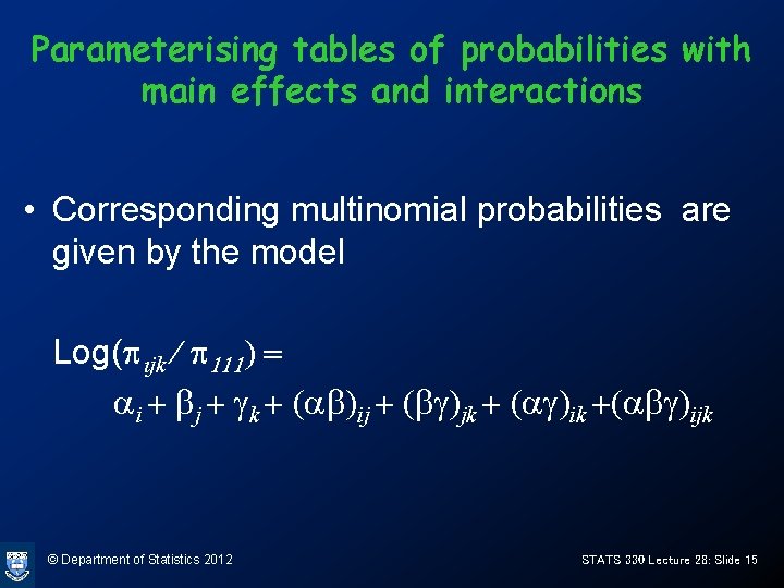
Parameterising tables of probabilities with main effects and interactions • Corresponding multinomial probabilities are given by the model Log(pijk / p 111) = ai + bj + gk + (ab)ij + (bg)jk + (ag)ik +(abg)ijk © Department of Statistics 2012 STATS 330 Lecture 28: Slide 15

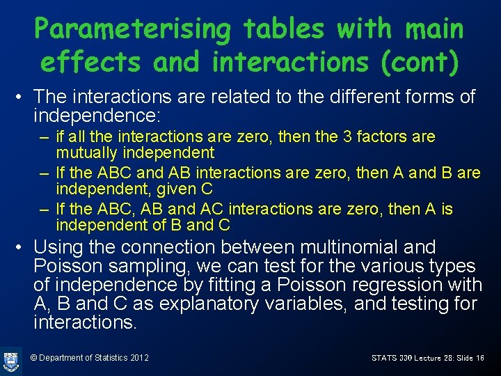
Parameterising tables with main effects and interactions (cont) • The interactions are related to the different forms of independence: – if all the interactions are zero, then the 3 factors are mutually independent – If the ABC and AB interactions are zero, then A and B are independent, given C – If the ABC, AB and AC interactions are zero, then A is independent of B and C • Using the connection between multinomial and Poisson sampling, we can test for the various types of independence by fitting a Poisson regression with A, B and C as explanatory variables, and testing for interactions. © Department of Statistics 2012 STATS 330 Lecture 28: Slide 16

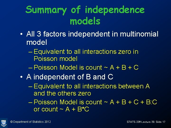
Summary of independence models • All 3 factors independent in multinomial model – Equivalent to all interactions zero in Poisson model – Poisson Model is count ~ A + B + C • A independent of B and C – Equivalent to all interactions between A and the others zero – Poisson Model is count ~ A + B + C + B: C or count ~ A + B*C © Department of Statistics 2012 STATS 330 Lecture 28: Slide 17

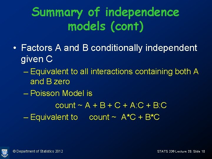
Summary of independence models (cont) • Factors A and B conditionally independent given C – Equivalent to all interactions containing both A and B zero – Poisson Model is count ~ A + B + C + A: C + B: C – Equivalent to count ~ A*C + B*C © Department of Statistics 2012 STATS 330 Lecture 28: Slide 18

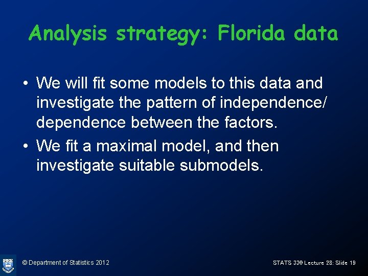
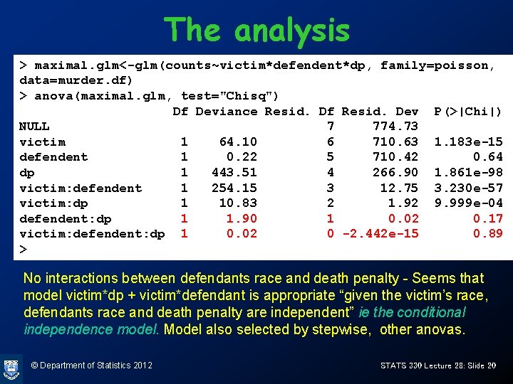
Analysis strategy: Florida data • We will fit some models to this data and investigate the pattern of independence/ dependence between the factors. • We fit a maximal model, and then investigate suitable submodels. © Department of Statistics 2012 STATS 330 Lecture 28: Slide 19

The analysis > maximal. glm<-glm(counts~victim*defendent*dp, family=poisson, data=murder. df) > anova(maximal. glm, test="Chisq") Df Deviance Resid. Df Resid. Dev P(>|Chi|) NULL 7 774. 73 victim 1 64. 10 6 710. 63 1. 183 e-15 defendent 1 0. 22 5 710. 42 0. 64 dp 1 443. 51 4 266. 90 1. 861 e-98 victim: defendent 1 254. 15 3 12. 75 3. 230 e-57 victim: dp 1 10. 83 2 1. 92 9. 999 e-04 defendent: dp 1 1. 90 1 0. 02 0. 17 victim: defendent: dp 1 0. 02 0 -2. 442 e-15 0. 89 > No interactions between defendants race and death penalty - Seems that model victim*dp + victim*defendant is appropriate “given the victim’s race, defendants race and death penalty are independent” ie the conditional independence model. Model also selected by stepwise, other anovas. © Department of Statistics 2012 STATS 330 Lecture 28: Slide 20

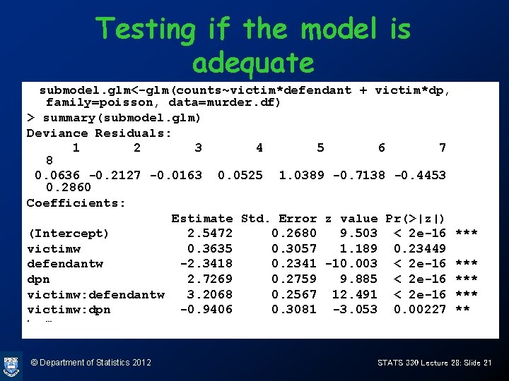
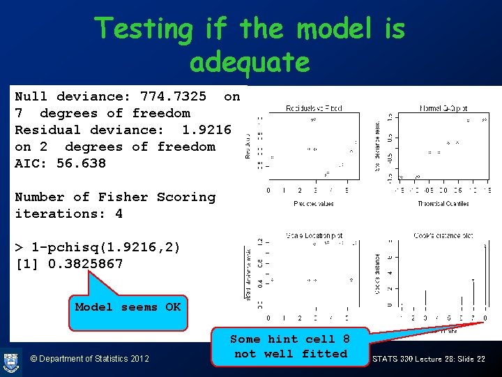
Testing if the model is adequate submodel. glm<-glm(counts~victim*defendant + victim*dp, family=poisson, data=murder. df) > summary(submodel. glm) Deviance Residuals: 1 2 3 4 5 6 7 8 0. 0636 -0. 2127 -0. 0163 0. 0525 1. 0389 -0. 7138 -0. 4453 0. 2860 Coefficients: Estimate Std. Error z value Pr(>|z|) (Intercept) 2. 5472 0. 2680 9. 503 < 2 e-16 *** victimw 0. 3635 0. 3057 1. 189 0. 23449 defendantw -2. 3418 0. 2341 -10. 003 < 2 e-16 *** dpn 2. 7269 0. 2759 9. 885 < 2 e-16 *** victimw: defendantw 3. 2068 0. 2567 12. 491 < 2 e-16 *** victimw: dpn -0. 9406 0. 3081 -3. 053 0. 00227 ** > • --- © Department of Statistics 2012 STATS 330 Lecture 28: Slide 21

Testing if the model is adequate Null deviance: 774. 7325 on 7 degrees of freedom Residual deviance: 1. 9216 on 2 degrees of freedom AIC: 56. 638 Number of Fisher Scoring iterations: 4 > 1 -pchisq(1. 9216, 2) [1] 0. 3825867 Model seems OK © Department of Statistics 2012 Some hint cell 8 not well fitted STATS 330 Lecture 28: Slide 22

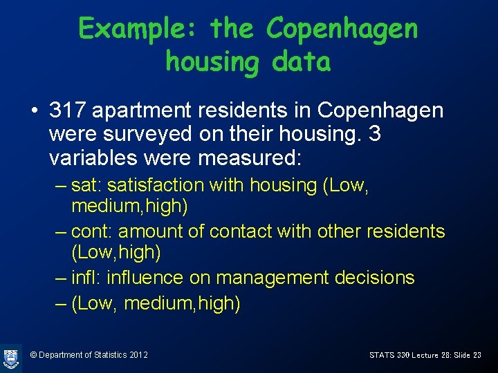
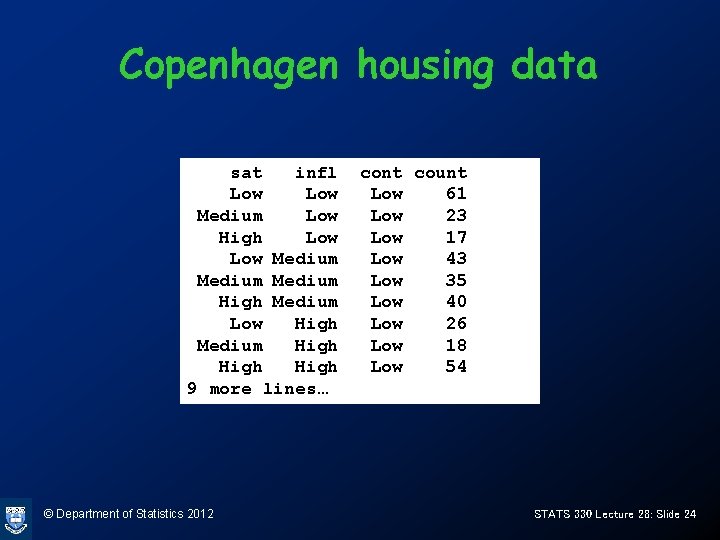
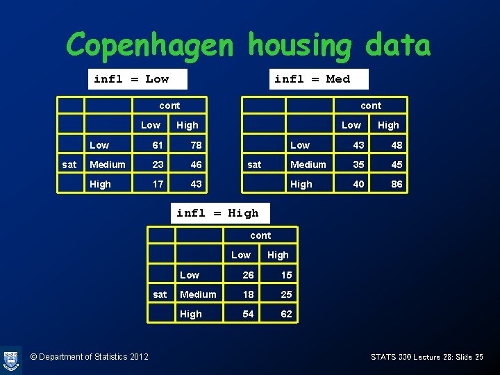
Example: the Copenhagen housing data • 317 apartment residents in Copenhagen were surveyed on their housing. 3 variables were measured: – sat: satisfaction with housing (Low, medium, high) – cont: amount of contact with other residents (Low, high) – infl: influence on management decisions – (Low, medium, high) © Department of Statistics 2012 STATS 330 Lecture 28: Slide 23

Copenhagen housing data sat infl Low Medium Low High Low Medium High Medium Low High Medium High 9 more lines… © Department of Statistics 2012 cont count Low 61 Low 23 Low 17 Low 43 Low 35 Low 40 Low 26 Low 18 Low 54 STATS 330 Lecture 28: Slide 24

Copenhagen housing data infl = Low Low 61 sat Medium High infl = Med cont 78 Low 43 48 23 46 sat Medium 35 45 17 43 High 40 86 Low High cont Low High infl = High © Department of Statistics 2012 cont Low 26 15 sat Medium 18 25 High 54 62 Low High STATS 330 Lecture 28: Slide 25

The analysis > housing. glm<-glm(count~sat*infl*cont, family=poisson, data=housing. df) > anova(housing. glm, test]”Chisq”) Df Deviance Resid. Df Resid. Dev P(>|Chi|) NULL 17 166. 757 sat 2 26. 191 15 140. 566 2. 054 e-06 infl 2 20. 040 13 120. 526 4. 451 e-05 cont 1 22. 544 12 97. 983 2. 054 e-06 sat: infl 4 75. 577 8 22. 406 1. 504 e-15 sat: cont 2 7. 745 6 14. 661 0. 021 infl: cont 2 11. 986 4 2. 675 0. 002 sat: infl: cont 4 2. 675 0 9. 546 e-15 0. 614 This time, only the 3 -factor interaction is insignificant. This is the “homogeneous association model” © Department of Statistics 2012 STATS 330 Lecture 28: Slide 26

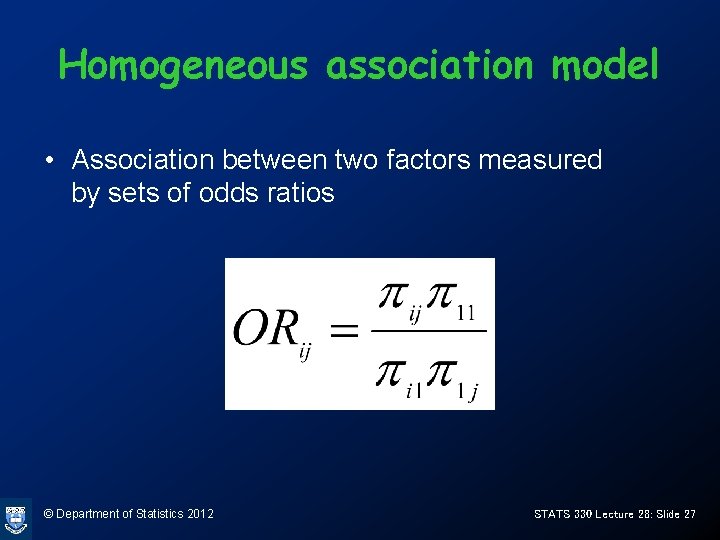
Homogeneous association model • Association between two factors measured by sets of odds ratios © Department of Statistics 2012 STATS 330 Lecture 28: Slide 27

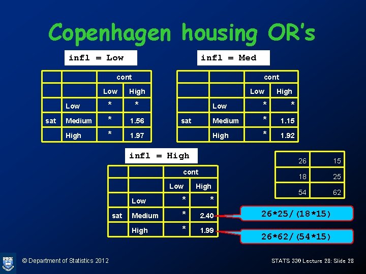
Copenhagen housing OR’s infl = Low infl = Med cont Low High Low * * sat Medium * 1. 56 sat Medium * 1. 15 High * 1. 97 High * 1. 92 infl = High © Department of Statistics 2012 cont Low * * sat Medium * 2. 40 High * 1. 99 Low High 26 15 18 25 54 62 26*25/(18*15) 26*62/(54*15) STATS 330 Lecture 28: Slide 28

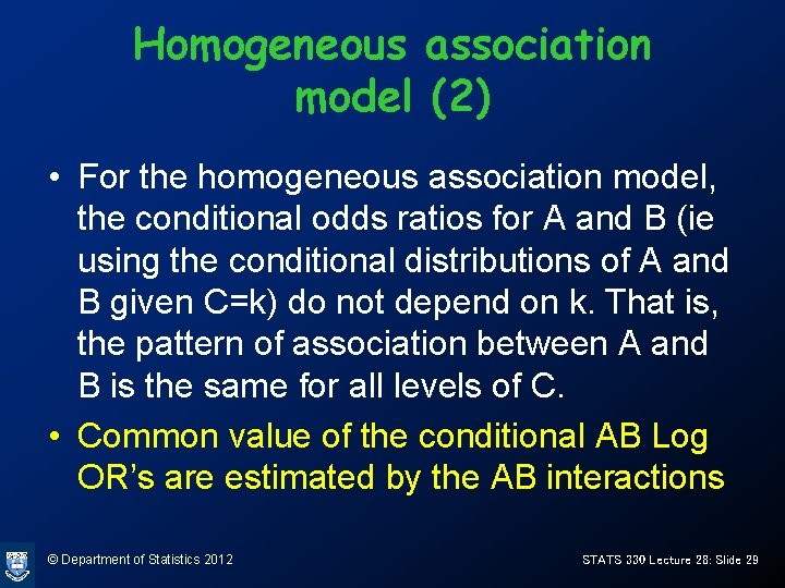
Homogeneous association model (2) • For the homogeneous association model, the conditional odds ratios for A and B (ie using the conditional distributions of A and B given C=k) do not depend on k. That is, the pattern of association between A and B is the same for all levels of C. • Common value of the conditional AB Log OR’s are estimated by the AB interactions © Department of Statistics 2012 STATS 330 Lecture 28: Slide 29

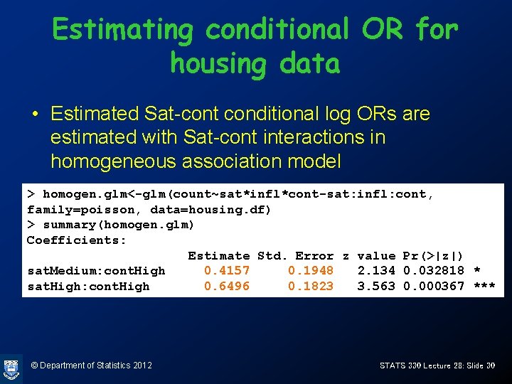
Estimating conditional OR for housing data • Estimated Sat-cont conditional log ORs are estimated with Sat-cont interactions in homogeneous association model > homogen. glm<-glm(count~sat*infl*cont-sat: infl: cont, family=poisson, data=housing. df) > summary(homogen. glm) Coefficients: Estimate Std. Error z value Pr(>|z|) sat. Medium: cont. High 0. 4157 0. 1948 2. 134 0. 032818 * sat. High: cont. High 0. 6496 0. 1823 3. 563 0. 000367 *** © Department of Statistics 2012 STATS 330 Lecture 28: Slide 30

Estimating conditional OR for housing data (2) > 0. 4157+c(-1, 1)*1. 96*0. 1948 [1] 0. 033892 0. 797508 > exp(0. 4157+c(-1, 1)*1. 96*0. 1948) [1] 1. 034473 2. 220002 > exp(0. 4157) [1] 1. 515431 > exp(0. 6496) [1] 1. 914775 • For med/High, est for log OR is 0. 4157, std error is 0. 1948 • CI for OR is exp(0. 4157 +/- 1. 96* 0. 1948) i. e. (1. 034, 2. 220) • Estimated OR for high/high is exp(0. 6496) = 1. 1914 © Department of Statistics 2012 STATS 330 Lecture 28: Slide 31

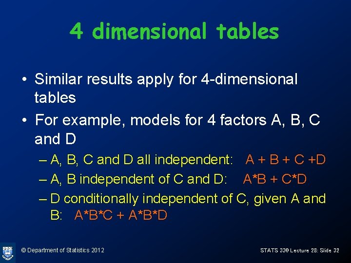
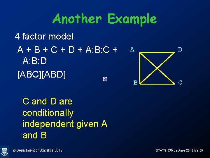
4 dimensional tables • Similar results apply for 4 -dimensional tables • For example, models for 4 factors A, B, C and D – A, B, C and D all independent: A + B + C +D – A, B independent of C and D: A*B + C*D – D conditionally independent of C, given A and B: A*B*C + A*B*D © Department of Statistics 2012 STATS 330 Lecture 28: Slide 32

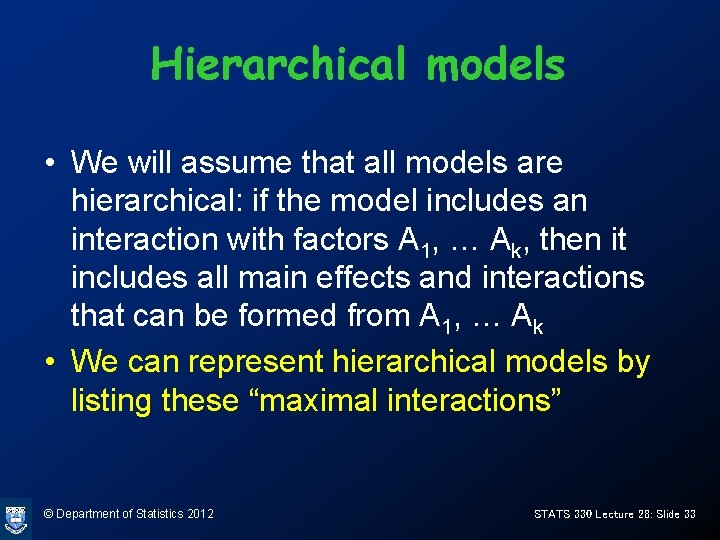
Hierarchical models • We will assume that all models are hierarchical: if the model includes an interaction with factors A 1, … Ak, then it includes all main effects and interactions that can be formed from A 1, … Ak • We can represent hierarchical models by listing these “maximal interactions” © Department of Statistics 2012 STATS 330 Lecture 28: Slide 33

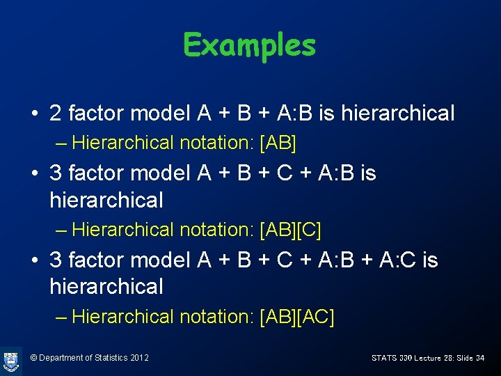
Examples • 2 factor model A + B + A: B is hierarchical – Hierarchical notation: [AB] • 3 factor model A + B + C + A: B is hierarchical – Hierarchical notation: [AB][C] • 3 factor model A + B + C + A: B + A: C is hierarchical – Hierarchical notation: [AB][AC] © Department of Statistics 2012 STATS 330 Lecture 28: Slide 34

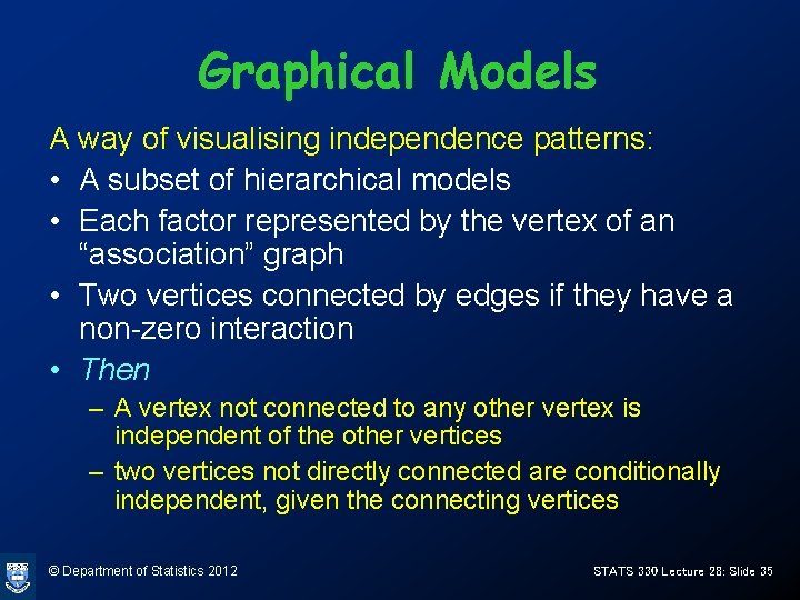
Graphical Models A way of visualising independence patterns: • A subset of hierarchical models • Each factor represented by the vertex of an “association” graph • Two vertices connected by edges if they have a non-zero interaction • Then – A vertex not connected to any other vertex is independent of the other vertices – two vertices not directly connected are conditionally independent, given the connecting vertices © Department of Statistics 2012 STATS 330 Lecture 28: Slide 35

Examples • 2 factor model A + B + A: B or [AB] A • 3 factor model A + B + C +AB or [AB][C] C independent of A and B • 3 factor model A + B + C + A: B + A: C +B: C or [AB][AC][BC] © Department of Statistics 2012 B A B C STATS 330 Lecture 28: Slide 36

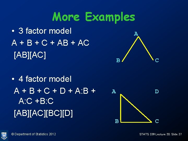
More Examples • 3 factor model A + B + C + AB + AC [AB][AC] • 4 factor model A + B + C + D + A: B + A: C +B: C [AB][AC][BC][D] A B © Department of Statistics 2012 C D C STATS 330 Lecture 28: Slide 37

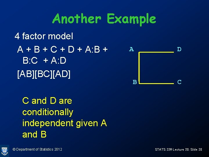
Another Example 4 factor model A + B + C + D + A: B + B: C + A: D [AB][BC][AD] A B D C C and D are conditionally independent given A and B © Department of Statistics 2012 STATS 330 Lecture 28: Slide 38

Another Example 4 factor model A + B + C + D + A: B: C + A: B: D [ABC][ABD] A B D C C and D are conditionally independent given A and B © Department of Statistics 2012 STATS 330 Lecture 28: Slide 39