Stats 330 Lecture 21 Department of Statistics 2012

Stats 330: Lecture 21 © Department of Statistics 2012 STATS 330 Lecture 21: Slide 1

Plan of the day In today’s lecture we continue our discussion of the logistic regression model Topics covered – Probabilities, odds & log odds – Inference for coefficients, probabilities and logodds – Calculating them in R • Reference: Coursebook, section 5. 2. 1 © Department of Statistics 2012 STATS 330 Lecture 21: Slide 2

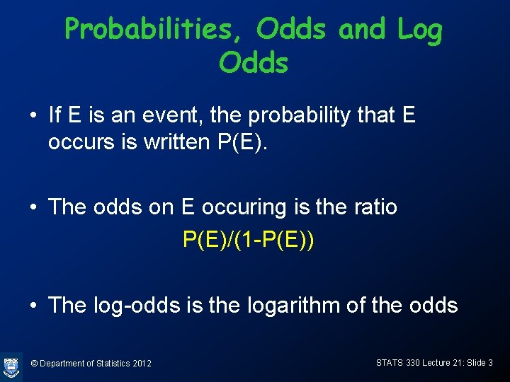
Probabilities, Odds and Log Odds • If E is an event, the probability that E occurs is written P(E). • The odds on E occuring is the ratio P(E)/(1 -P(E)) • The log-odds is the logarithm of the odds © Department of Statistics 2012 STATS 330 Lecture 21: Slide 3

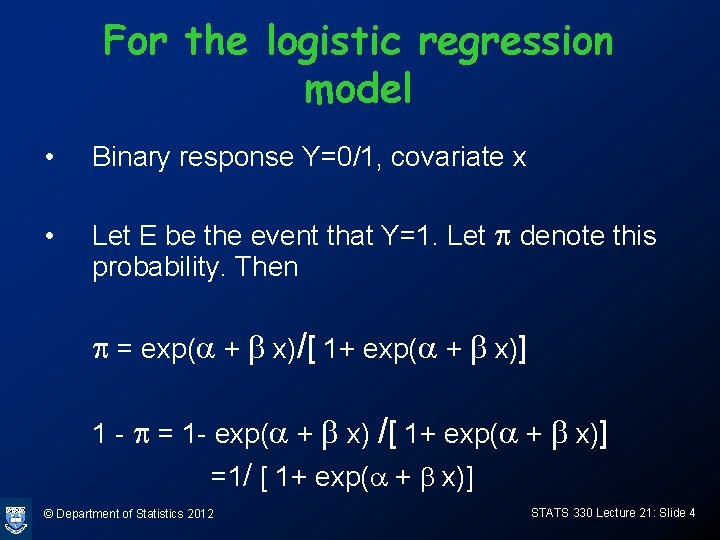
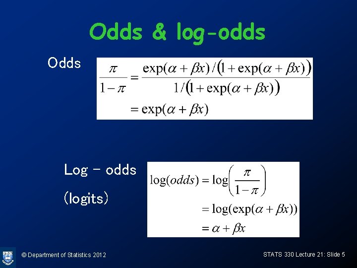
For the logistic regression model • Binary response Y=0/1, covariate x • Let E be the event that Y=1. Let p denote this probability. Then p = exp(a + b x)/[ 1+ exp(a + b x)] 1 - p = 1 - exp(a + b x) /[ 1+ exp(a + b x)] =1/ [ 1+ exp(a + b x)] © Department of Statistics 2012 STATS 330 Lecture 21: Slide 4

Odds & log-odds Odds Log – odds (logits) © Department of Statistics 2012 STATS 330 Lecture 21: Slide 5

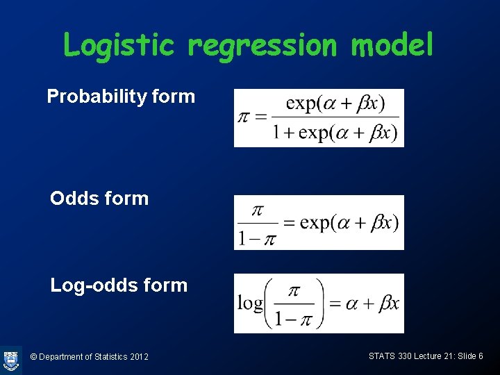
Logistic regression model Probability form Odds form Log-odds form © Department of Statistics 2012 STATS 330 Lecture 21: Slide 6

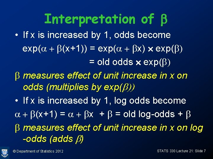
Interpretation of b • If x is increased by 1, odds become exp(a + b(x+1)) = exp(a + bx) ´ exp(b) = old odds ´ exp(b) b measures effect of unit increase in x on odds (multiplies by exp(b)) • If x is increased by 1, log odds become a + b(x+1) = a + bx + b = old log-odds + b b measures effect of unit increase in x on log -odds (adds b) © Department of Statistics 2012 STATS 330 Lecture 21: Slide 7

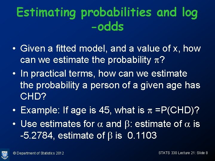
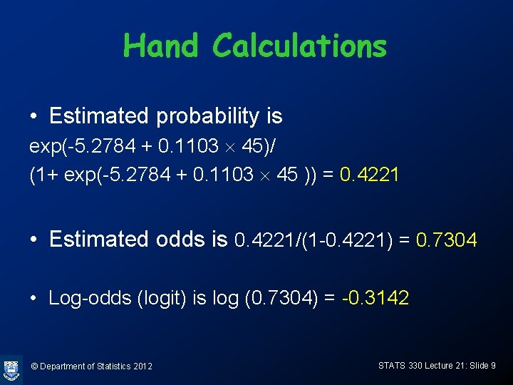
Estimating probabilities and log -odds • Given a fitted model, and a value of x, how can we estimate the probability p? • In practical terms, how can we estimate the probability a person of a given age has CHD? • Example: If age is 45, what is p =P(CHD)? • Use estimates for a and b: estimate of a is -5. 2784, estimate of b is 0. 1103 © Department of Statistics 2012 STATS 330 Lecture 21: Slide 8

Hand Calculations • Estimated probability is exp(-5. 2784 + 0. 1103 ´ 45)/ (1+ exp(-5. 2784 + 0. 1103 ´ 45 )) = 0. 4221 • Estimated odds is 0. 4221/(1 -0. 4221) = 0. 7304 • Log-odds (logit) is log (0. 7304) = -0. 3142 © Department of Statistics 2012 STATS 330 Lecture 21: Slide 9

Calculations using R > predict(chd. glm, data. frame(age=45), type="response") Calculates [1] 0. 4221367 probability > predict(chd. glm, data. frame(age=45)) [1] -0. 314008 Calculates logodds © Department of Statistics 2012 STATS 330 Lecture 21: Slide 10

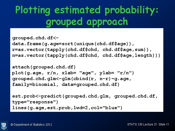
Plotting estimated probability: grouped approach grouped. chd. df<data. frame(g. age=sort(unique(chd. df$age)), r=as. vector(tapply(chd. df$chd, chd. df$age, sum)), n=as. vector(tapply(chd. df$chd, chd. df$age, length))) attach(grouped. chd. df) plot(g. age, r/n, xlab= "age", ylab= "r/n") grouped. chd. glm<-glm(cbind(r, n-r)~g. age, family=binomial, data=grouped. chd. df) est. prob<-predict(grouped. chd. glm, grouped. chd. df, type="response") lines(g. age, est. prob, lwd=2, col="blue") © Department of Statistics 2012 STATS 330 Lecture 21: Slide 11

© Department of Statistics 2012 STATS 330 Lecture 21: Slide 12

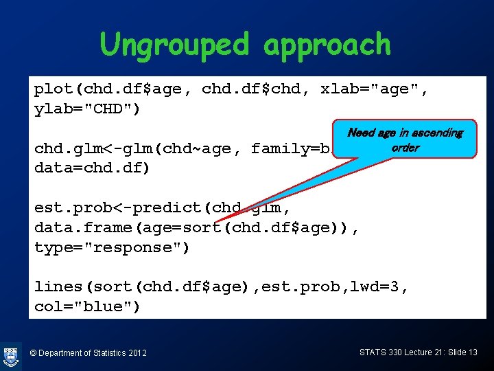
Ungrouped approach plot(chd. df$age, chd. df$chd, xlab="age", ylab="CHD") chd. glm<-glm(chd~age, data=chd. df) Need age in ascending order family=binomial, est. prob<-predict(chd. glm, data. frame(age=sort(chd. df$age)), type="response") lines(sort(chd. df$age), est. prob, lwd=3, col="blue") © Department of Statistics 2012 STATS 330 Lecture 21: Slide 13

© Department of Statistics 2012 STATS 330 Lecture 21: Slide 14

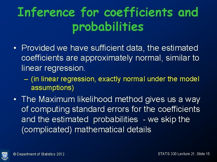
Inference for coefficients and probabilities • Provided we have sufficient data, the estimated coefficients are approximately normal, similar to linear regression. – (in linear regression, exactly normal under the model assumptions) • The Maximum likelihood method gives us a way of computing standard errors for the coefficients and the estimated probabilities - we skip the (complicated) mathematical details © Department of Statistics 2012 STATS 330 Lecture 21: Slide 15

Testing for a zero coefficient • To test if a coefficient is zero we use the tstatistic and p-value just as in linear regression – tests are interpreted the same way • (in the case of a single covariate, this is testing that there is no relationship between covariate and response) © Department of Statistics 2012 STATS 330 Lecture 21: Slide 16

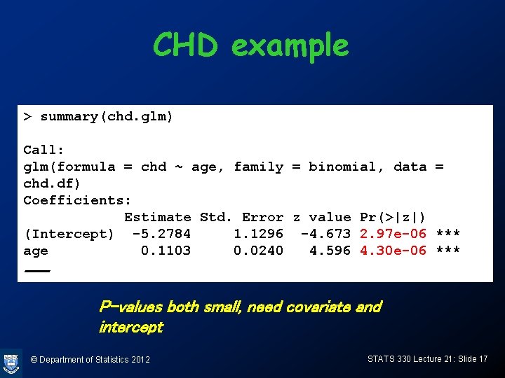
CHD example > summary(chd. glm) Call: glm(formula = chd ~ age, family = binomial, data = chd. df) Coefficients: Estimate Std. Error z value Pr(>|z|) (Intercept) -5. 2784 1. 1296 -4. 673 2. 97 e-06 *** age 0. 1103 0. 0240 4. 596 4. 30 e-06 *** --P-values both small, need covariate and intercept © Department of Statistics 2012 STATS 330 Lecture 21: Slide 17

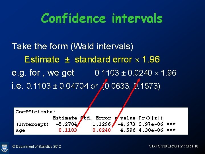
Confidence intervals Take the form (Wald intervals) Estimate ± standard error ´ 1. 96 e. g. for , we get 0. 1103 ± 0. 0240 ´ 1. 96 i. e. 0. 1103 ± 0. 04704 or (0. 0633, 0. 1573) Coefficients: Estimate Std. Error z value Pr(>|z|) (Intercept) -5. 2784 1. 1296 -4. 673 2. 97 e-06 *** age 0. 1103 0. 0240 4. 596 4. 30 e-06 *** © Department of Statistics 2012 STATS 330 Lecture 21: Slide 18

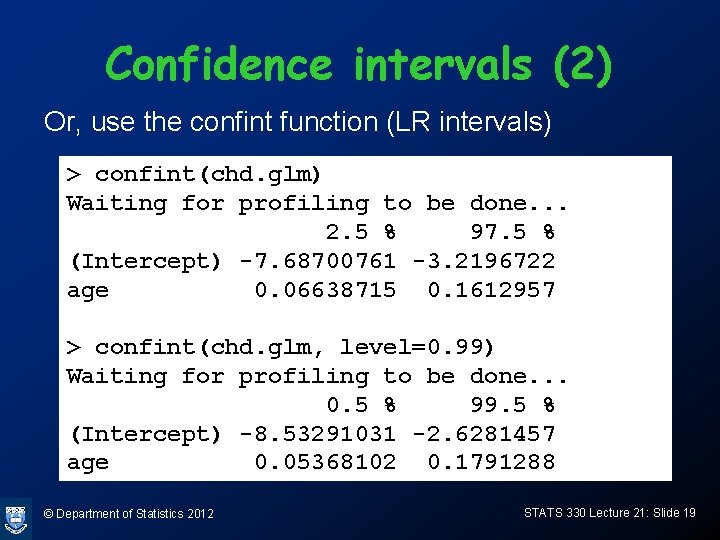
Confidence intervals (2) Or, use the confint function (LR intervals) > confint(chd. glm) Waiting for profiling to be done. . . 2. 5 % 97. 5 % (Intercept) -7. 68700761 -3. 2196722 age 0. 06638715 0. 1612957 > confint(chd. glm, level=0. 99) Waiting for profiling to be done. . . 0. 5 % 99. 5 % (Intercept) -8. 53291031 -2. 6281457 age 0. 05368102 0. 1791288 © Department of Statistics 2012 STATS 330 Lecture 21: Slide 19

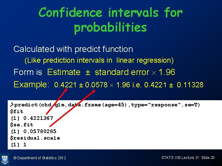
Confidence intervals for probabilities Calculated with predict function (Like prediction intervals in linear regression) Form is Estimate ± standard error ´ 1. 96 Example: 0. 4221 ± 0. 0578 ´ 1. 96 i. e. 0. 4221 ± 0. 11328 > predict(chd. glm, data. frame(age=45), type="response", se=T) $fit [1] 0. 4221367 $se. fit [1] 0. 05780285 $residual. scale [1] 1 © Department of Statistics 2012 STATS 330 Lecture 21: Slide 20

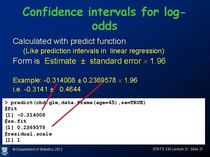
Confidence intervals for logodds Calculated with predict function (Like prediction intervals in linear regression) Form is Estimate ± standard error ´ 1. 96 Example: -0. 314008 ± 0. 2369578 ´ 1. 96 i. e. -0. 3141 ± 0. 4644 > predict(chd. glm, data. frame(age=45), se=TRUE) $fit [1] -0. 314008 $se. fit [1] 0. 2369578 $residual. scale [1] 1 © Department of Statistics 2012 STATS 330 Lecture 21: Slide 21

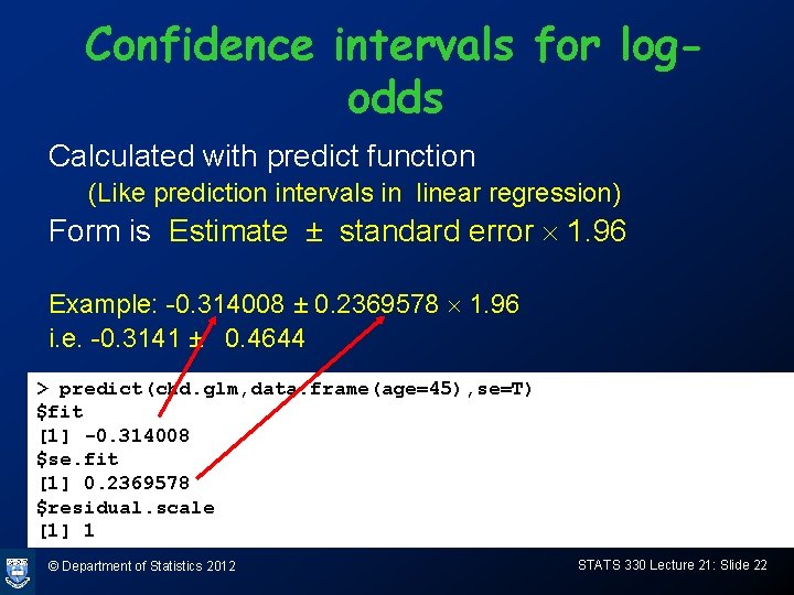
Confidence intervals for logodds Calculated with predict function (Like prediction intervals in linear regression) Form is Estimate ± standard error ´ 1. 96 Example: -0. 314008 ± 0. 2369578 ´ 1. 96 i. e. -0. 3141 ± 0. 4644 > predict(chd. glm, data. frame(age=45), se=T) $fit [1] -0. 314008 $se. fit [1] 0. 2369578 $residual. scale [1] 1 © Department of Statistics 2012 STATS 330 Lecture 21: Slide 22