Statistics Statistical Process Control Control Charting Cayman Systems

Statistics Statistical Process Control & Control Charting © Cayman Systems USA 513 777 -3394 Revision A 19991008 - www. 16949. com Statistical Analysis and SPC Slide 1

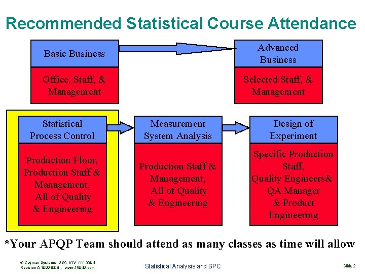
Recommended Statistical Course Attendance Basic Business Advanced Business Office, Staff, & Management Selected Staff, & Management Statistical Process Control Production Floor, Production Staff & Management, All of Quality & Engineering Measurement System Analysis Design of Experiment Production Staff & Management, All of Quality & Engineering Specific Production Staff, Quality Engineers& QA Manager & Product Engineering *Your APQP Team should attend as many classes as time will allow © Cayman Systems USA 513 777 -3394 Revision A 19991008 - www. 16949. com Statistical Analysis and SPC Slide 2

Basic Definitions Statistics: the science of collecting, analyzing, interpreting and presenting data. A Statistic is a single characteristic taken from this process. © Cayman Systems USA 513 777 -3394 Revision A 19991008 - www. 16949. com Statistical Analysis and SPC Slide 3

Universe, Populations & Samples Universe: the collection of all elements Population: the set of objects of interest Sample: a subset of objects taken from the population Randam Sample: all possible samples of the same size have an equal chance of occuring. © Cayman Systems USA 513 777 -3394 Revision A 19991008 - www. 16949. com Statistical Analysis and SPC Slide 4

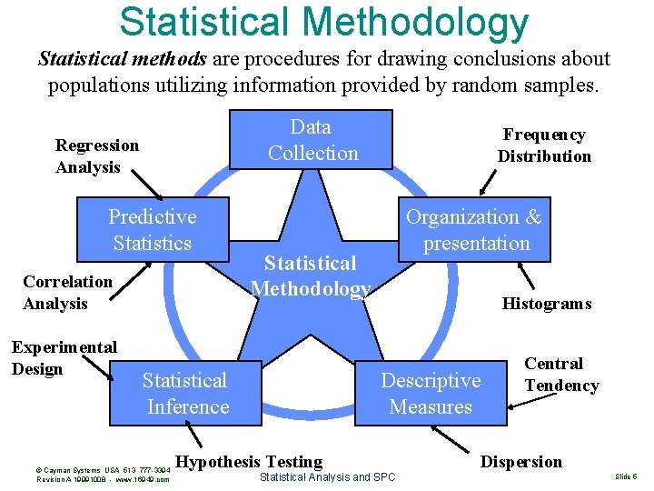
Statistical Methodology Statistical methods are procedures for drawing conclusions about populations utilizing information provided by random samples. Data Collection Regression Analysis Predictive Statistics Correlation Analysis Experimental Design Organization & presentation Statistical Methodology Statistical Inference © Cayman Systems USA 513 777 -3394 Revision A 19991008 - www. 16949. com Frequency Distribution Histograms Descriptive Measures Hypothesis Testing Statistical Analysis and SPC Central Tendency Dispersion Slide 5

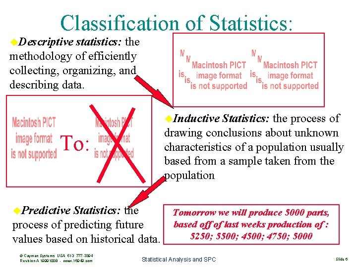
Classification of Statistics: Descriptive statistics: the methodology of efficiently collecting, organizing, and describing data. Inductive Statistics: the process of drawing conclusions about unknown characteristics of a population usually based from a sample taken from the population To: Predictive Statistics: the process of predicting future values based on historical data. © Cayman Systems USA 513 777 -3394 Revision A 19991008 - www. 16949. com Tomorrow we will produce 5000 parts, based off of last weeks production of : 5250; 5500; 4750; 5000 Statistical Analysis and SPC Slide 6

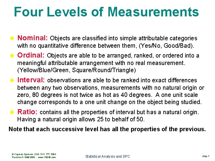
Four Levels of Measurements Nominal: Objects are classified into simple attributable categories with no quantitative difference between them, (Yes/No, Good/Bad). Ordinal: Objects are able to be arranged, ranked, or ordered into a meaningful attributable arrangement with no real measurement. (Yellow/Blue/Green, Square/Round/Triangle) Interval: observations are able to be ranked into exact differences between any two observations, measurements with no natural origin or zero, 80 degrees is not twice as hot as 40 degrees. A one unit scale change corresponds to a one unit change on the object being studied. Ratio: contains all the properties of interval but has a natural origin. Having a natural origin allows 25 to behalf of 50. Note that each successive level has all the properties of the previous. © Cayman Systems USA 513 777 -3394 Revision A 19991008 - www. 16949. com Statistical Analysis and SPC Slide 7

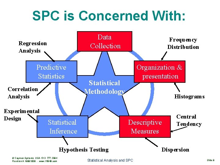
SPC is Concerned With: Data Collection Regression Analysis Predictive Statistics Correlation Analysis Experimental Design Frequency Distribution Organization & presentation Statistical Methodology Statistical Inference Histograms Descriptive Measures Hypothesis Testing © Cayman Systems USA 513 777 -3394 Revision A 19991008 - www. 16949. com Statistical Analysis and SPC Central Tendency Dispersion Slide 8

Data Collection © Cayman Systems USA 513 777 -3394 Revision A 19991008 - www. 16949. com Statistical Analysis and SPC Slide 9

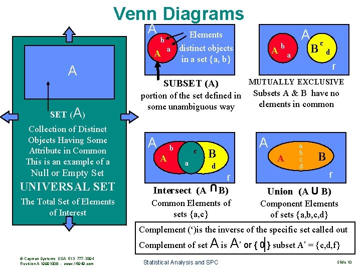
Venn Diagrams A A A SET (A) Collection of Distinct Objects Having Some Attribute in Common This is an example of a Null or Empty Set A Elements b a distinct objects in a set {a, b} portion of the set defined in some unambiguous way b A c a a B c d f MUTUALLY EXCLUSIVE SUBSET (A) A A b Subsets A & B have no elements in common A B A d a b c d B f f B) Union (A U B) UNIVERSAL SET Intersect (A The Total Set of Elements of Interest Common Elements of sets {a, c} Component Elements of sets {a, b, c, d} U Complement (‘)is the inverse of the specific set called out Complement of set A is A’ or { 0 } subset A’ = {c, d, f} © Cayman Systems USA 513 777 -3394 Revision A 19991008 - www. 16949. com Statistical Analysis and SPC Slide 10

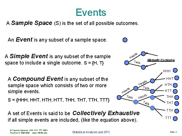
Events A Sample An Space (S) is the set of all possible outcomes. Event is any subset of a sample space. s ad e H A Simple Event is any subset of the sample space to include a single outcome. S = {H, T} Mutually Exclusive Tails HHH A Compound Event is any subset of the sample space which consists of two or more simple events. S = {HHH, HHT, HTH, HTT, THH, THT, TTH, TTT} H ds a He Tails Statistical Analysis and SPC Tails ds Hea Tail A set of Events is said to be Collectively Exhaustive if all simple events are included, (like the equation above). © Cayman Systems USA 513 777 -3394 Revision A 19991008 - www. 16949. com HHT s ead HTH HTT THH s THT TTH TTT Slide 11

Putting it all Together When gathering data for a process, we must realize that © Cayman Systems USA 513 777 -3394 Revision A 19991008 - www. 16949. com Statistical Analysis and SPC Slide 12

Organizing Data © Cayman Systems USA 513 777 -3394 Revision A 19991008 - www. 16949. com Statistical Analysis and SPC Slide 13

Presenting Data © Cayman Systems USA 513 777 -3394 Revision A 19991008 - www. 16949. com Statistical Analysis and SPC Slide 14

SPC Statistical Process Control The development and use of statistics and statistical theories about distributions and how they vary has become the corner stone of process improvement. Statistical process control allows the user to continuously monitor, analyze, and control the process. SPC is based on the understanding of variation and how it effects the output of any process. Variation is the amount of deviation from a design nominal value. Not every product that is produced will exactly match it's design nominal values. That's why we have tolerances on the nominal values to judge whether a product is acceptable or not. But the closer we are to the nominal value the better the product is. Control charts are one SPC tool that enables us to monitor and control process variation. © Cayman Systems USA 513 777 -3394 Revision A 19991008 - www. 16949. com Statistical Analysis and SPC Slide 15

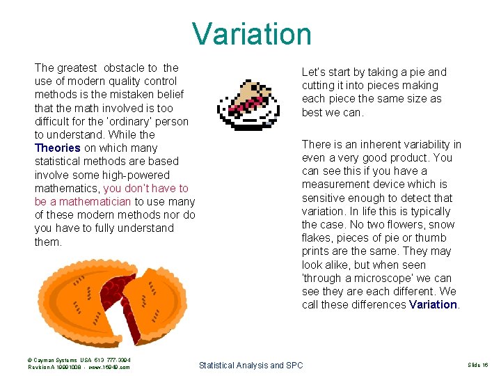
Variation The greatest obstacle to the use of modern quality control methods is the mistaken belief that the math involved is too difficult for the ‘ordinary’ person to understand. While the Theories on which many statistical methods are based involve some high-powered mathematics, you don’t have to be a mathematician to use many of these modern methods nor do you have to fully understand them. © Cayman Systems USA 513 777 -3394 Revision A 19991008 - www. 16949. com Let’s start by taking a pie and cutting it into pieces making each piece the same size as best we can. There is an inherent variability in even a very good product. You can see this if you have a measurement device which is sensitive enough to detect that variation. In life this is typically the case. No two flowers, snow flakes, pieces of pie or thumb prints are the same. They may look alike, but when seen ‘through a microscope’ we can see they are each different. We call these differences Variation. Statistical Analysis and SPC Slide 16

Causes of Variation Special Causes of Variation Common Causes of Variation Special causes are problems that arise in a periodic fashion. They are somewhat unpredictable and can be dealt with at the machine or operator level. Examples of special causes are operator error, broken tools, and machine setting drift. This type of variation is not critical and only represents a small fraction of the variation found in a process. Common causes are problems inherent in the system itself. They are always present and effect the output of the process. Examples of common causes of variation are poor training, inappropriate production methods, and poor workstation design. As we can see, common causes of variation are more critical on the manufacturing process than special causes. In fact Dr. Deming suggests that about 80 to 85% of all the problems encountered in production processes are caused by common causes, while only 15 to 20% are caused by special causes © Cayman Systems USA 513 777 -3394 Revision A 19991008 - www. 16949. com Statistical Analysis and SPC Slide 17

Causes of Variation Special Causes of Variation Common Causes of Variation +Accounts for 5 -15% of quality problems. +Is due to a factor that has "slipped" into the process causing unstable or unpredictable variation. +Are unpredictable variations that are abnormal to the process including human error, equipment failure, defective/changed raw materials, acid spills, power failures, etc. ; failure to remove them can result is corrosion, scale, metal fatigue, lower equipment efficiency, increased maintenance costs, unsafe working conditions, wasted chemicals, increased down-time (plant shut-down. . . ), etc. +Removal of all special causes of variation yields a process that is in statistical control. +Correctable by local personnel. +Account for 85 -95% of quality problems +Are due to the many small sources of variation "engineered" into the process of the "system”. +Are naturally caused and are always present in the process because they are linked to the system's base ability to perform; it is the predictable and stable inherent variability resulting from the process operating as it was designed. +Standard deviation, s, is used as a measure of the inherent process variability; it helps describe the well-known normal distribution curve. +Correctable only by management; typically requires the repair/replacement of a system's component, or the system itself. © Cayman Systems USA 513 777 -3394 Revision A 19991008 - www. 16949. com Statistical Analysis and SPC Slide 18

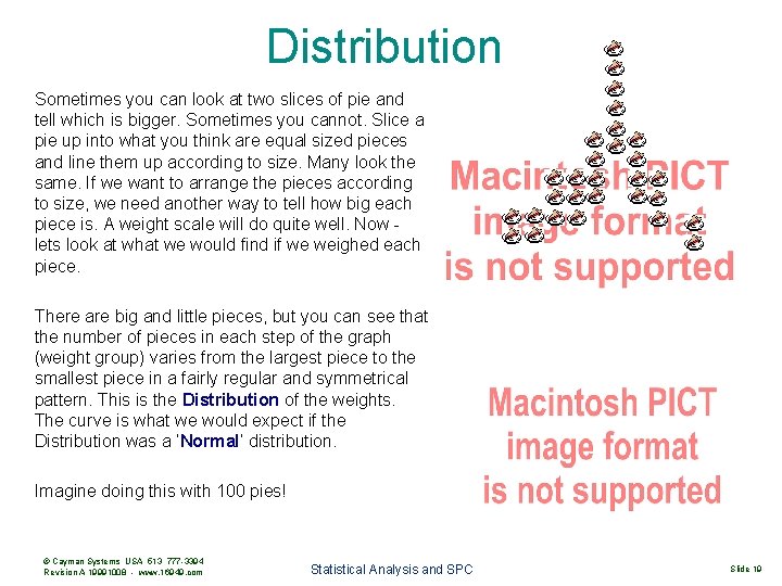
Distribution Sometimes you can look at two slices of pie and tell which is bigger. Sometimes you cannot. Slice a pie up into what you think are equal sized pieces and line them up according to size. Many look the same. If we want to arrange the pieces according to size, we need another way to tell how big each piece is. A weight scale will do quite well. Now lets look at what we would find if we weighed each piece. There are big and little pieces, but you can see that the number of pieces in each step of the graph (weight group) varies from the largest piece to the smallest piece in a fairly regular and symmetrical pattern. This is the Distribution of the weights. The curve is what we would expect if the Distribution was a ‘Normal’ distribution. Imagine doing this with 100 pies! © Cayman Systems USA 513 777 -3394 Revision A 19991008 - www. 16949. com Statistical Analysis and SPC Slide 19

A ‘Normal’ Distribution © Cayman Systems USA 513 777 -3394 Revision A 19991008 - www. 16949. com Statistical Analysis and SPC Slide 20

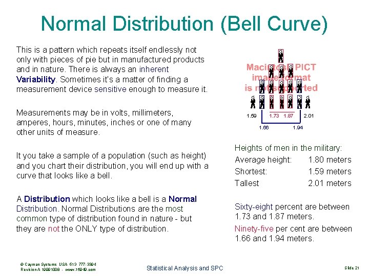
Normal Distribution (Bell Curve) This is a pattern which repeats itself endlessly not only with pieces of pie but in manufactured products and in nature. There is always an inherent Variability. Sometimes it’s a matter of finding a measurement device sensitive enough to measure it. Measurements may be in volts, millimeters, amperes, hours, minutes, inches or one of many other units of measure. It you take a sample of a population (such as height) and you chart their distribution, you will end up with a curve that looks like a bell. A Distribution which looks like a bell is a Normal Distributions are the most common type of distribution found in nature - but they are not the ONLY type of distribution. © Cayman Systems USA 513 777 -3394 Revision A 19991008 - www. 16949. com Statistical Analysis and SPC 1. 59 1. 73 1. 87 1. 66 2. 01 1. 94 Heights of men in the military: Average height: 1. 80 meters Shortest: 1. 59 meters Tallest 2. 01 meters Sixty-eight percent are between 1. 73 and 1. 87 meters. Ninety-five per cent are between 1. 66 and 1. 94 meters. Slide 21

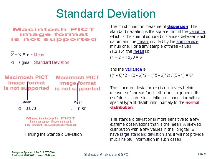
Standard Deviation The most common measure of dispersion. The standard deviation is the square root of the variance, which is the sum of squared distances between each datum and the mean, divided by the sample size minus one. For a tiny sample of three values (1, 2, 15), the mean is: (1 + 2 + 15)/3 = 6 X = X-Bar = Mean s = sigma = Standard Deviation and the variance is ((1 - 6)^2 + (2 - 6)^2 + (15 - 6)^2) / (3 - 1) = 61 Mean s = 0. 070 s = 0. 80 Finding the Standard Deviation © Cayman Systems USA 513 777 -3394 Revision A 19991008 - www. 16949. com The standard deviation (s) is not a very helpful measure of spread for distributions in general. Its usefulness is due to its intimate connection with a special type of distribution, namely to the normal distribution. The standard deviation is more sensitive to a few extreme observations than is the mean. A skewed distribution with a few values in the 'long tail' will have large standard deviation and it will not provide much helpful information in such cases. Statistical Analysis and SPC Slide 22

Standard Deviation © Cayman Systems USA 513 777 -3394 Revision A 19991008 - www. 16949. com Statistical Analysis and SPC Slide 23

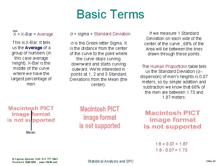
Basic Terms X = X-Bar = Average This is X-Bar. It tells us the Average of a group of numbers (in this case average height). X-Bar is the middle of the curve where we have the largest percentage of men. s = sigma = Standard Deviation s is the Greek letter Sigma. It is the distance from the center of the curve to the point where the curve stops curving downward and starts curving outward. We’re interested in points at 1, 2 and 3 Standard Deviations from the Mean (the center). If we measure 1 Standard Deviation on each side of the center of the curve , 68% of the Area will be between the lines drawn through these points. The Human Proportions table tells us the Standard Deviation (s dispersion) of men’s heights is 0. 07 meters, so by simple addition and subtraction we know that 68% of the men are between 1. 73 and 1. 87 meters. Mean 1. 8 + 0. 07 = 1. 87 1. 8 - 0. 07 = 1. 73 © Cayman Systems USA 513 777 -3394 Revision A 19991008 - www. 16949. com Statistical Analysis and SPC Slide 24

More On Standard Deviation Two Standard Deviations Two standard deviations would be 0. 14 meters. Ninety-five percent of men are between 1. 66 and 1. 94 meters. Three Standard Deviations are s = 0. 07 x 2 = 0. 14 0. 21 meters and 99. 73% of the Area of the Normal curve is between +3 1. 8 - 0. 14 = 1. 66 sigma (+3 s) and -3 s. We can say that practically all of the men are 1. 8 + 0. 14 = 1. 94 between 1. 59 and 2. 01 meters. Only about 13 in 10, 000 men are taller than 2. 01 meters. The same is true of men below 1. 59 meters. But… Three Standard Deviations s = 0. 07 x 3 = 0. 21 1. 8 - 0. 21 = 1. 59 1. 8 + 0. 21 = 2. 01 What does this have to do with making nuts, bolts, transmissions and aspirin tablets? If we have a machine which will measure every man who comes down the street, what are the odds that any individual man is 1. 8 meters tall? What are the odds that the next man who walks by will be between 1. 59 and 2. 01 meters? How about between 1. 73 and 1. 87 meters? © Cayman Systems USA 513 777 -3394 Revision A 19991008 - www. 16949. com Statistical Analysis and SPC Slide 25

Dispersion Revisited Sixty-eight % of all men are between 1. 73 and 1. 87 meters tall. So, there are 68 chances in 100 that the next man will be between these Limits. I’d have to give you odds of 68 to 32 (2: 1). Ninety-five % of all men are between 1. 66 and 1. 94 meters tall. That gives us odds of 95 to 5 (19: 1) that the next man won’t be shorter than 1. 66 nor taller than 1. 94 meters. There are only 2 1/2 chances in 100 that the next man will be taller than 1. 94 meters and 13 1/2 chances in 10, 000 (1: 740) that he will be taller than 2. 01 meters. The gadgets we make are supposed to be exactly 20 millimeters long. We are going to make a Lot of 500 widgets. We measure the Lot with a micrometer and find: As you can see, they are in the same Bell Shaped Pattern as the pieces of pie and the men. © Cayman Systems USA 513 777 -3394 Revision A 19991008 - www. 16949. com Statistical Analysis and SPC Slide 26

Population vs Sample The Average is 20 millimeters, but individually they vary from 19. 10 mm to 20. 90 mm. This is OK with our customers because their specification calls for and Average of 20 mm with a Tolerance of +/-1. 5 mm. That means they will accept anything between 18. 5 and 21. 5 mm. These points are know as the Limits or the Tolerance Limits. Our problem is to keep the widget cutting machines at the center of 20. 0 mm and to not let individuals vary (disperse) more than they did in this lot. All of the gadgets we measured were made at one time (the same Run) on the same machine by the same operator and from the same material lot. Because of all these things being the same, we can be quite sure that the Pattern of their Variation will almost exactly fit the Normal Curve. We would also know that the greatest Individual Variations will be quite close to +/-3 s. This is a Spread of 6 Standard Deviations. © Cayman Systems USA 513 777 -3394 Revision A 19991008 - www. 16949. com Statistical Analysis and SPC The difference between the Longest (20. 9 mm) and the Shortest (19. 1 mm) is 1. 80 mm. One sixth of 1. 80 is 0. 3. So…. The standard deviation is 0. 3 mm. Since we measured every widget, we measured the entire Population. We can do the same thing with a Sample. Slide 27

Samples To take a sample, you take gadgets out of a bucket. A Sample is usually more than 1 piece. We’ll use a Sample Size of 5. BUT WAIT!!! We want a Random Sample. To get a Random Sample we must ‘dig around’ in the bucket we’re taking gadgets from. If we do this 5 times, we shold see something like the table below. These 5 Sample Averages vary quite a bit from the Lot Average of 20. 0 mm, but the Grand Average is 20. 01 mm. We wouldn’t always come so close, but if we have enough Samples (say 20 to 25) the Average of a number of Samples will be a good Estimate of the Actual Average of the Lot. You’ll notice the table has another number labeled Range. The range is the difference between the largest and smallest measurement in each sample. Like the Averages, the Ranges vary in each sample. © Cayman Systems USA 513 777 -3394 Revision A 19991008 - www. 16949. com Statistical Analysis and SPC Slide 28

Samples In our Lot of 500 gadgets we divided the Range by 6 to get the Standard Deviation. In that case we were measuring a Population. We can’t do that with Samples of 5 because we had 500 chances of getting some of the extreme values - not just 5 chances. In Samples of 5 there is less chance of getting some of the extreme values so the Divisor will be smaller. We call this divisor the d 2 (d two) factor. We can find (look up) the appropriate d factor in a Table. For a sample size of 5, the d 2 factor is 2. 326 (from the table). Dividing the Average Range (0. 734) by the d 2 factor (2. 326) gives us a Standard Deviation of 0. 316. This doesn’t differ much from the figure of 0. 3 which we got when we measured 500 pieces. This shows that by taking relatively small samples we can Estimate two very important things about the Distribution of the Measurements of any product: The Average and the Standard Deviation. X = X-Bar = Average s = sigma = Standard Deviation The Standard Deviation (s) of the gadgets is 0. 3 mm and the Average is 20. 00 mm. Knowing these 2 values, we can now put some % figures on our Normal Distribution Curve. If we’re doing a good job of cutting the gadgets to the Average of 20 mm, 68% should be between 19. 70 and 20. 30 mm. Ninety-five percent should be between -2 s and +2 s (19. 40 mm and 20. 90 mm). 99. 73% should be between -3 s and +3 s (19. 10 mm and 20. 90 mm). © Cayman Systems USA 513 777 -3394 Revision A 19991008 - www. 16949. com Statistical Analysis and SPC Slide 29

Samples Even if something very unusual happens to give me an occasional gadget shorter than 19. 10 mm, or longer than 20. 90 mm, as long as the gadget machine is properly adjusted to make an Average of 20. 00 mm I could give you odds of 997 to 3 that you can’t find one (At Random) outside of these Limits. But - You and I know that machines, materials and operators do not always do what they are supposed to do. © Cayman Systems USA 513 777 -3394 Revision A 19991008 - www. 16949. com Statistical Analysis and SPC Slide 30

Samples Bill Jones works on machine #2. Bill’s mother-in-law has been camping at his house for the last 6 weeks. Bill has been feeling sort of frustrated. His mind just isn’t focused on cutting gadgets. Yesterday his machine was off about four tenths (4/10) of a millimeter. How did we find out? We cannot if we just look at a few individual gadgets. Let’s assume that his Average was 20. 40 mm. The Pattern of the Variation of Individual Measurements about the center of the 20. 40 mm was the same as in any good lot… Except - the Bell Shaped Curve was shoved over +0. 40 mm. Sigma (Standard Deviation) is the same (0. 3 mm). The 3 s Limits of his Distribution are now changed to 19. 50 mm and 21. 30 mm. They are within the customer’s specification of 18. 50 mm through 21. 50 mm… But - the customer will probably complain about the higher Average. We’ve already seen that a good Lot can be expected to vary between 19. 10 mm and 20. 90 mm. Five per cent of the gadgets Bill was making were over the limit of 20. 90 mm. NOTE: You have top use a Statistical Table to figure this out! If we were to pick up single pieces from Bill’s machine, there are only 5 chances in 100, or 1 chance in 20, that we would get one of the pieces which is larger than 20. 90 mm. © Cayman Systems USA 513 777 -3394 Revision A 19991008 - www. 16949. com Statistical Analysis and SPC Slide 31

So What? Remember a while back we gave Odds of 740 to 1 that the next man to walk by the height machine would not be taller than 2. 01 meters. We were betting that he would not exceed the 3 sigma Limit. What if we look at the next 2 men who walk by. It’s a safe bet that the Average of the two will be nearer the Grand Average of 1. 80 meters than to the extreme height of 2. 01 meters. For the same Odds of 740: 1, I’d have to use narrower 3 sigma (s) Limits. If we bet on the Average of the next 4 men, we’d have to use still narrower Limits? No! These Limits are NOT reduced in proportion to the number of men (the Sample Size). Limits for the Average of 2 men would be about 2/3 of the Limits for Individuals. For the Average of 4 men, the Limits would be 1/2 the Limits for Individuals. How do we get these figures? Not only do measurements of Individuals vary in the Bell Shaped Pattern of the Norman Distribution Curve, but Sample Averages vary in the same Pattern, about the same Center. However, the Standard Deviation (sigma or s) of Sample Averages is the s of Individuals divided by the Square Root of the Sample Size. In the case of our men, the Sigma of Individual Heights is 0. 07 meters. For each Sample size we divide 0. 07 m by the Square Root of the Sample Size. © Cayman Systems USA 513 777 -3394 Revision A 19991008 - www. 16949. com Statistical Analysis and SPC Slide 32

A Square Root? We get Square Roots from a Table or a Calculator. Let’s apply this principle to measuring gadgets from Bill’s machine. We take Samples of 5 gadgets from the machine every 15 minutes and measure them with a dial micrometer. We have seen that Standard Deviation (sigma or s) of this measurement is 0. 3 mm. The Square Root of 5 (the Sample Size) is 2. 236. Dividing 0. 3 by 2. 236 gives us a Standard Deviation of 0. 134 mm for Averages of 5 gadgets. 3 Standard Deviations is 0. 402 mm. 0. 3 mm / √ 5 = 0. 134 mm (Adjustment for Sample Size) 3 x 0. 134 mm = 0. 402 mm (Yields the Spread) © Cayman Systems USA 513 777 -3394 Revision A 19991008 - www. 16949. com Statistical Analysis and SPC Slide 33

A Shift in the Center If Bill’s machine is set up right, for an Average of 20. 00 mm, Averages of 5 should not vary more than 0. 4 mm above and below this Center (between 19. 60 mm and 20. 40 mm). As long as our Sample Averages vary between these limits we can be reasonably sure that the Actual Average of the machine is close to the Specified Average of 20. 00 mm. It’s a 740: 1 bet that no Sample Average is higher than 20. 40 mm. But… If Bill’s machine setting is 20. 40 mm, Averages of Samples of 5 will vary 0. 4 mm on either side of this High Center. There is now a 50: 50 chance that any Sample Average will be above 20. 40 mm. Of course, there’s the same 50: 50 chance that the Sample Average will be BELOW 20. 40 mm. But… With these Odds in our favour we’re practically certain to get a high Average in the first 2 or 3 Samples. © Cayman Systems USA 513 777 -3394 Revision A 19991008 - www. 16949. com Statistical Analysis and SPC Slide 34

Control Chart Developed in the mid 1920's by Walter Shewhart of Bell labs, this SPC tool has become a major contributor to the quality improvement process. It allows the use to monitor and control process variation. It also allow the user to make the proper corrective actions to eliminate the sources of variation. Even though they require the user to have some statistical background, the are relatively easy to construct. There are two basic types of control charts, the average and range control charts. The first deals with how close the process is to the nominal design value, while the range chart indicates the amount of spread or variability around the nominal design value. A control chart has basically three lines: the upper control limit UCL, the center line CL (average), and the lower control limit LCL. These lines are computed from samples taken from the production line. Each sample represents a point on the control chart. A minimum of 25 points is required for a control chart to be accurate. In the Control Chart at the right, the Center Line says that the gadgets should Average 20. 00 mm. The Upper and Lower dotted lines say that if this specification is met, Averages of Sample sizes (n) of 5 (n = 5) should not be less than 19. 60 mm nor more than 20. 40 mm. © Cayman Systems USA 513 777 -3394 Revision A 19991008 - www. 16949. com A Control Chart is a Picture of what we are doing. Upper Control Limit X Control Chart of Gadgets Sample Size (n) = 5 Lower Control Limit Average Statistical Analysis and SPC What’s Wrong With This Picture? Slide 35

Control Charts Serve 2 Basic Purposes Control Charts provide information for decision making with respect to a manufacturing process. When a random pattern of variation occurs and process capability has been established, the process should be left alone. When an unstable (nonrandom) pattern of variation is occurring, action should be taken to find and eliminate the disturbing or assignable causes. * Control Charts provide information for decision making with respect to recently produced product. The Control Chart can be used as one source of information in the determination of whether product should be released to the customer or some alternate disposition made. * © Cayman Systems USA 513 777 -3394 Revision A 19991008 - www. 16949. com Statistical Analysis and SPC Slide 36

Control Charts The most common type of Control Chart is the X-Bar & R Chart X = X-Bar = Average © Cayman Systems USA 513 777 -3394 Revision A 19991008 - www. 16949. com Statistical Analysis and SPC Slide 37

Control Chart Construction Don’t Forget The ‘Details’ !!! 1. Take measurements of the characteristic being studied. More ‘Details’ !!! Lowest value Highest value X = X-Bar = Average 3. Calculate subgroup average X-Bar Sum of values divided by number of samples (n) 187 / 5 = 37. 4 4. Calculate Range Highest value - Lowest value 43 -31=12 © Cayman Systems USA 513 777 -3394 Revision A 19991008 - www. 16949. com Statistical Analysis and SPC 2. Calculate sum of measurements Add up sample values 33+38+31+43+42 Slide 38

Control Chart Construction 5. Plot Data (!) 45 44 43 42 41 40 39 38 37 36 35 34 33 32 31 30 55 50 45 40 35 30 25 20 15 10 5 © Cayman Systems USA 513 777 -3394 Revision A 19991008 - www. 16949. com • • Statistical Analysis and SPC Slide 39

Chart the Data • 1. Continue plotting data. … 2. Connect the dots !!! • • © Cayman Systems USA 513 777 -3394 Revision A 19991008 - www. 16949. com • • • • Statistical Analysis and SPC Slide 40

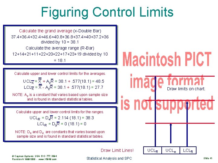
Figuring Control Limits Calculate the grand average (x-Double Bar) 37. 4+36. 4+32. 4+46. 6+40. 8+36. 8+37. 4+40+37. 2+36 divided by 10 = 38. 1 Calculate the average range (R-Bar) 12+14+21+11+22+20+22+17+23+19 divided by 10 = 18. 1 Calculate upper and lower control limits for the averages. UCLX = X + A 2 R = 38. 1 +. 577(18. 1) = 48. 5 LCLX = X - A 2 R = 38. 1 +. 577(18. 1) = 27. 7 Draw limits on chart. NOTE: A 2 is a constant that varies based upon sample size and is found in standard statistical tables. Calculate upper and lower control limits for the ranges. UCLR = D 4 R = 2. 114 (18. 1) = 38. 3 LCLR = D 3 R = 0 (18. 1) = 0 NOTE: D 3 and D 4 are constants that varies based upon sample size and is found in standard statistical tables. Draw Limit Lines! © Cayman Systems USA 513 777 -3394 Revision A 19991008 - www. 16949. com Statistical Analysis and SPC UCLX UCLR LCLX Slide 41

A 1, D 3 and D 4 Table A Note: These numbers often vary slightly from table to table. © Cayman Systems USA 513 777 -3394 Revision A 19991008 - www. 16949. com Statistical Analysis and SPC Slide 42

Attribute Control Charts © Cayman Systems USA 513 777 -3394 Revision A 19991008 - www. 16949. com Statistical Analysis and SPC Slide 43

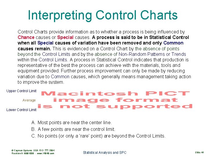
Interpreting Control Charts provide information as to whether a process is being influenced by Chance causes or Special causes. A process is said to be in Statistical Control when all Special causes of variation have been removed and only Common causes remain. This is evidenced on a Control Chart by the absence of points beyond the Control Limits and by the absence of Non-Random Patterns or Trends within the Control Limits. A process in Statistical Control indicates that production is representative of the best the process can achieve with the materials, tools and equipment provided. Further process improvement can only be made by reducing variation due to Common causes, which generally means management taking action to improve the system. Upper Control Limit Average Lower Control Limit A. Most points are near the center line. B. A few points are near the control limit. C. No points (or only a ‘rare’ point) are beyond the Control Limits. © Cayman Systems USA 513 777 -3394 Revision A 19991008 - www. 16949. com Statistical Analysis and SPC Slide 44

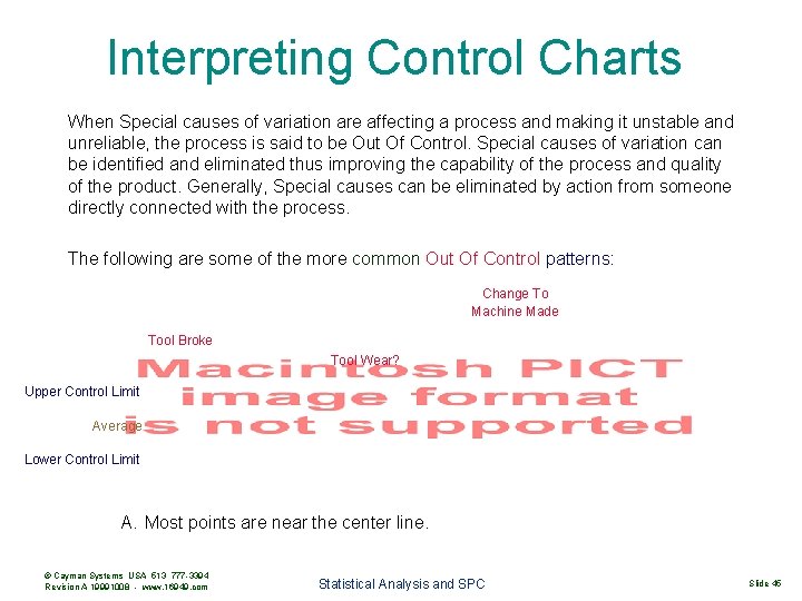
Interpreting Control Charts When Special causes of variation are affecting a process and making it unstable and unreliable, the process is said to be Out Of Control. Special causes of variation can be identified and eliminated thus improving the capability of the process and quality of the product. Generally, Special causes can be eliminated by action from someone directly connected with the process. The following are some of the more common Out Of Control patterns: Change To Machine Made Tool Broke Tool Wear? Upper Control Limit Average Lower Control Limit A. Most points are near the center line. © Cayman Systems USA 513 777 -3394 Revision A 19991008 - www. 16949. com Statistical Analysis and SPC Slide 45

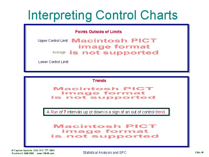
Interpreting Control Charts Points Outside of Limits Upper Control Limit Average Lower Control Limit Trends A Run of 7 intervals up or down is a sign of an out of control trend. © Cayman Systems USA 513 777 -3394 Revision A 19991008 - www. 16949. com Statistical Analysis and SPC Slide 46

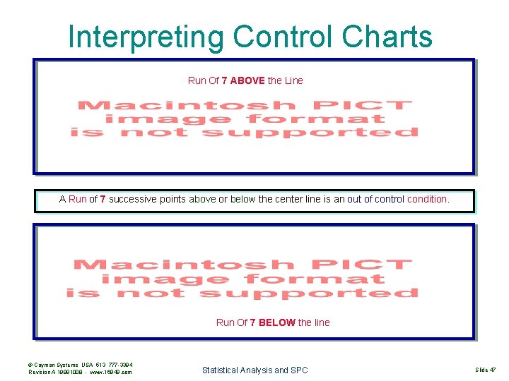
Interpreting Control Charts Run Of 7 ABOVE the Line A Run of 7 successive points above or below the center line is an out of control condition. Run Of 7 BELOW the line © Cayman Systems USA 513 777 -3394 Revision A 19991008 - www. 16949. com Statistical Analysis and SPC Slide 47

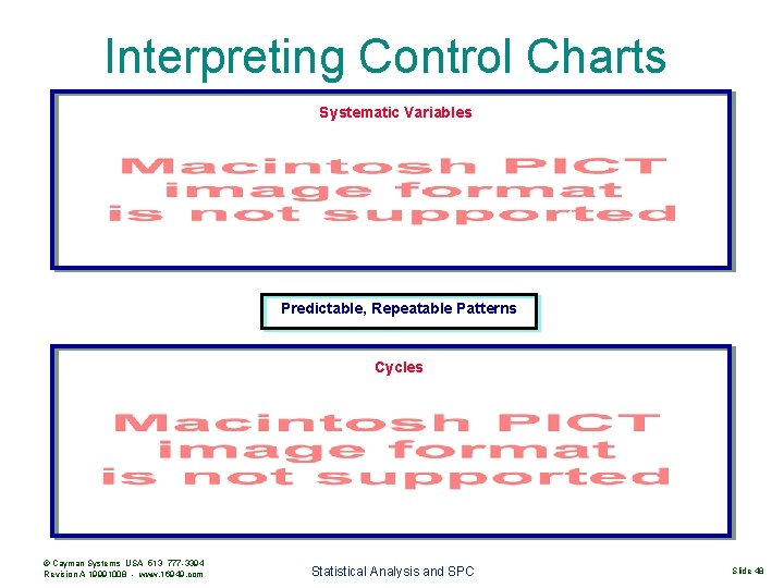
Interpreting Control Charts Systematic Variables Predictable, Repeatable Patterns Cycles © Cayman Systems USA 513 777 -3394 Revision A 19991008 - www. 16949. com Statistical Analysis and SPC Slide 48

Interpreting Control Charts Freaks Sudden, Unpredictable Instability Large Fluctuations, Erratic Up and Down Movements © Cayman Systems USA 513 777 -3394 Revision A 19991008 - www. 16949. com Statistical Analysis and SPC Slide 49

Interpreting Control Charts Mixtures Unusual Number of Points Near Control Limits (Different Machines? ) Sudden Shift in Level Typically Indicates a Change in the System or Process © Cayman Systems USA 513 777 -3394 Revision A 19991008 - www. 16949. com Statistical Analysis and SPC Slide 50

Interpreting Control Charts Stratification Constant, Small Fluctuations Near the Center of the Chart xxxxxx ccccccc © Cayman Systems USA 513 777 -3394 Revision A 19991008 - www. 16949. com Statistical Analysis and SPC Slide 51

Interpreting Control Charts Drift Sharp Breaks. Various Possible Causes Cyclical Possible Environmental (Seasonal? ) Fluctuations © Cayman Systems USA 513 777 -3394 Revision A 19991008 - www. 16949. com Statistical Analysis and SPC Slide 52

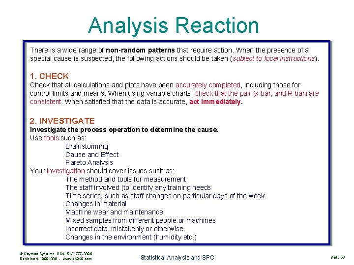
Analysis Reaction There is a wide range of non-random patterns that require action. When the presence of a special cause is suspected, the following actions should be taken (subject to local instructions). 1. CHECK Check that all calculations and plots have been accurately completed, including those for control limits and means. When using variable charts, check that the pair (x bar, and R bar) are consistent. When satisfied that the data is accurate, act immediately. 2. INVESTIGATE Investigate the process operation to determine the cause. Use tools such as: Brainstorming Cause and Effect Pareto Analysis Your investigation should cover issues such as: The method and tools for measurement The staff involved (to identify any training needs Time series, such as staff changes on particular days of the week Changes in material Machine wear and maintenance Mixed samples from different people or machines Incorrect data, mistakenly or otherwise Changes in the environment (humidity etc. ) © Cayman Systems USA 513 777 -3394 Revision A 19991008 - www. 16949. com Statistical Analysis and SPC Slide 53

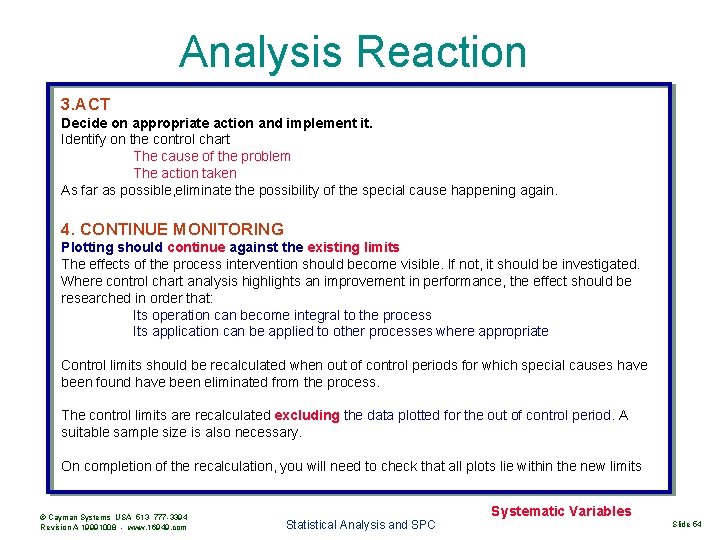
Analysis Reaction 3. ACT Decide on appropriate action and implement it. Identify on the control chart The cause of the problem The action taken As far as possible, eliminate the possibility of the special cause happening again. 4. CONTINUE MONITORING Plotting should continue against the existing limits The effects of the process intervention should become visible. If not, it should be investigated. Where control chart analysis highlights an improvement in performance, the effect should be researched in order that: Its operation can become integral to the process Its application can be applied to other processes where appropriate Control limits should be recalculated when out of control periods for which special causes have been found have been eliminated from the process. The control limits are recalculated excluding the data plotted for the out of control period. A suitable sample size is also necessary. On completion of the recalculation, you will need to check that all plots lie within the new limits © Cayman Systems USA 513 777 -3394 Revision A 19991008 - www. 16949. com Statistical Analysis and SPC Systematic Variables Slide 54