Standard Trend Models Trend Curves Purposes of a





- Slides: 19

Standard Trend Models

Trend Curves • Purposes of a Trend Curve: 1. Forecasting the long run 2. Estimating the growth rate

Standard Trend Curves • Key Properties: – have a simple form – have good track records – software for fitting is widely available

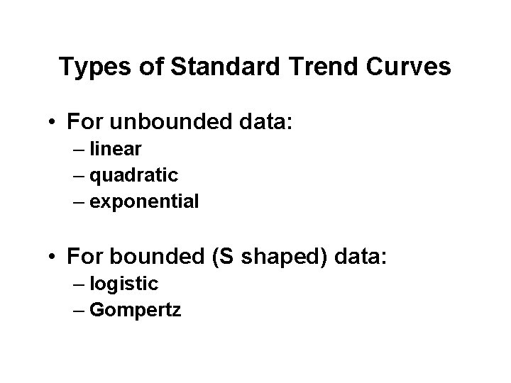
Types of Standard Trend Curves • For unbounded data: – linear – quadratic – exponential • For bounded (S shaped) data: – logistic – Gompertz

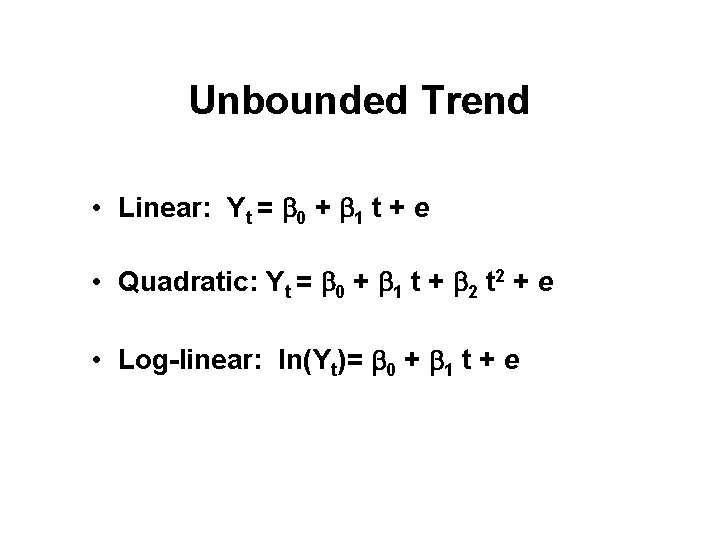
Unbounded Trend • Linear: Yt = b 0 + b 1 t + e • Quadratic: Yt = b 0 + b 1 t + b 2 t 2 + e • Log-linear: ln(Yt)= b 0 + b 1 t + e

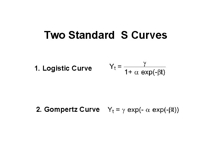
Two Standard S Curves 1. Logistic Curve 2. Gompertz Curve

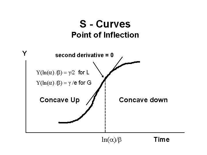
S – Curves (Life Cycle Theory) 4 Stages of New Technology Life Cycle 1. Slow growth at the beginning stage 2. Rapid growth 3. Slow growth during the mature stage 4. Decline during the final stage

S - Curves Point of Inflection Y second derivative = 0 Y(ln(a) /b) = g/2 for L Y(ln(a) /b) = g /e for G Concave Up Concave down ln(a)/b Time

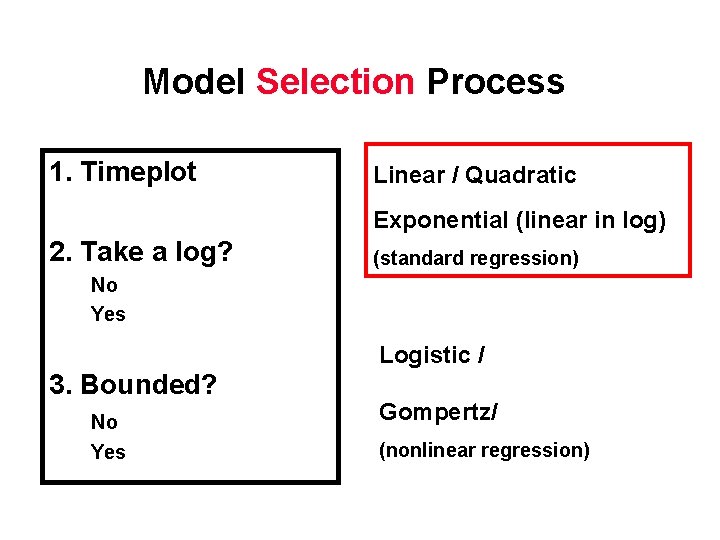
Model Selection Process 1. Timeplot Linear / Quadratic Exponential (linear in log) 2. Take a log? (standard regression) No Yes Logistic / 3. Bounded? No Yes Gompertz/ (nonlinear regression)

Nonlinear Least Squares • SPSS is one of the few statistics packages that provide routines for fitting nonlinear regression models. • You have to provide initial estimates for parameters.

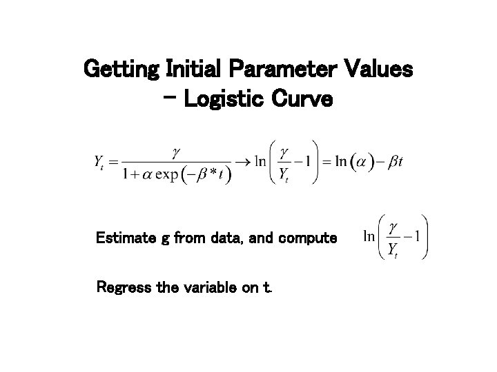
Getting Initial Parameter Values - Logistic Curve Estimate g from data, and compute Regress the variable on t.

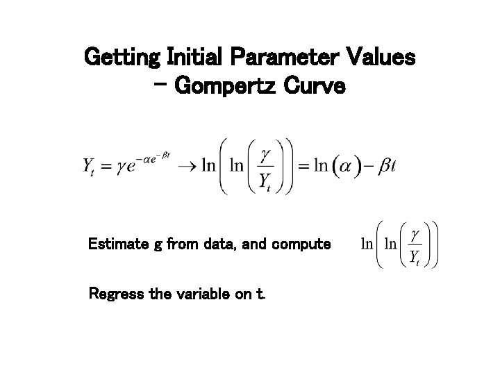
Getting Initial Parameter Values - Gompertz Curve Estimate g from data, and compute Regress the variable on t.

Durbin-Watson Test

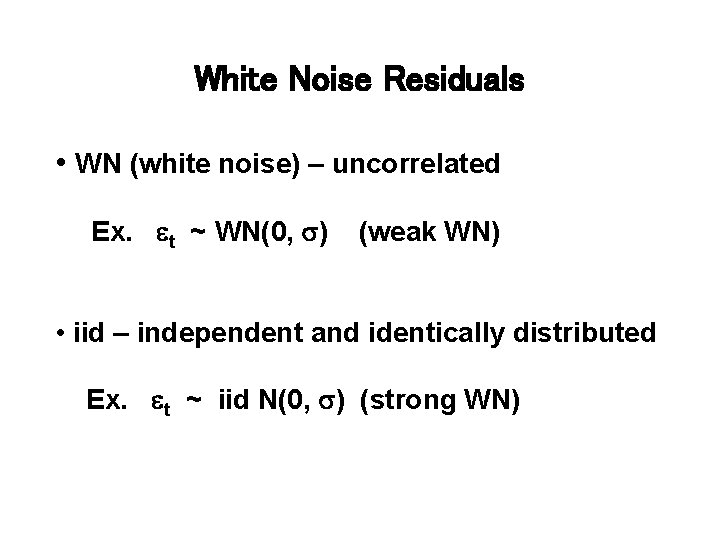
White Noise Residuals • WN (white noise) – uncorrelated Ex. et ~ WN(0, s) (weak WN) • iid – independent and identically distributed Ex. et ~ iid N(0, s) (strong WN)

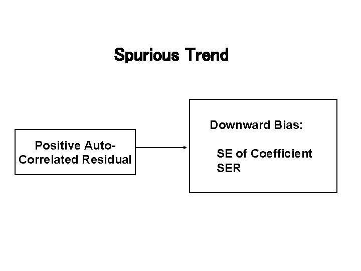
Spurious Trend Downward Bias: Positive Auto. Correlated Residual SE of Coefficient SER

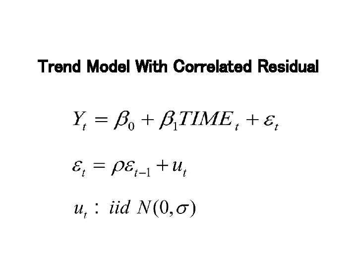
Trend Model With Correlated Residual

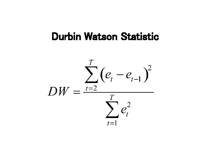
Durbin Watson Statistic

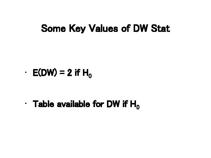
Some Key Values of DW Stat • E(DW) = 2 if H 0 • Table available for DW if H 0

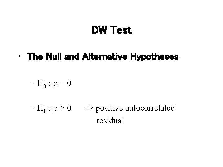
DW Test • The Null and Alternative Hypotheses – H 0 : r = 0 – H 1 : r > 0 -> positive autocorrelated residual