Signal Linear system Chapter 3 Time Domain Analysis
![3. 2 Useful Signal Operations Time Shift Signal x[n ± 1] represents instant shifted 3. 2 Useful Signal Operations Time Shift Signal x[n ± 1] represents instant shifted](https://slidetodoc.com/presentation_image_h2/3f9313562ab36b47b73feb4ff5439580/image-10.jpg)
![3. 2 Useful Signal Operations Time- Reversal (Flip) Signal x[-n] represents flip version of 3. 2 Useful Signal Operations Time- Reversal (Flip) Signal x[-n] represents flip version of](https://slidetodoc.com/presentation_image_h2/3f9313562ab36b47b73feb4ff5439580/image-12.jpg)
![3. 2 Useful Signal Operations Time-scale Find f[2 k], f[k/2] Basil Hamed 13 3. 2 Useful Signal Operations Time-scale Find f[2 k], f[k/2] Basil Hamed 13](https://slidetodoc.com/presentation_image_h2/3f9313562ab36b47b73feb4ff5439580/image-13.jpg)
![3. 3 Some Useful Discrete-time Signal Models Discrete-Time Unit Step Function u[n] u[n-k]= Basil 3. 3 Some Useful Discrete-time Signal Models Discrete-Time Unit Step Function u[n] u[n-k]= Basil](https://slidetodoc.com/presentation_image_h2/3f9313562ab36b47b73feb4ff5439580/image-16.jpg)
![3. 3 Some Useful Discrete-time Signal Models Discrete-Time Unit ramp Function r[n]= Basil Hamed 3. 3 Some Useful Discrete-time Signal Models Discrete-Time Unit ramp Function r[n]= Basil Hamed](https://slidetodoc.com/presentation_image_h2/3f9313562ab36b47b73feb4ff5439580/image-17.jpg)
![3. 3 Some Useful Discrete-time Signal Models D-T Sinusoids X[n]=Acos (Ω n+ θ) Use 3. 3 Some Useful Discrete-time Signal Models D-T Sinusoids X[n]=Acos (Ω n+ θ) Use](https://slidetodoc.com/presentation_image_h2/3f9313562ab36b47b73feb4ff5439580/image-18.jpg)
![3. 5 DT System Equations: Now…isolating the y[n] term gives the “Recursive Form”: “current” 3. 5 DT System Equations: Now…isolating the y[n] term gives the “Recursive Form”: “current”](https://slidetodoc.com/presentation_image_h2/3f9313562ab36b47b73feb4ff5439580/image-30.jpg)
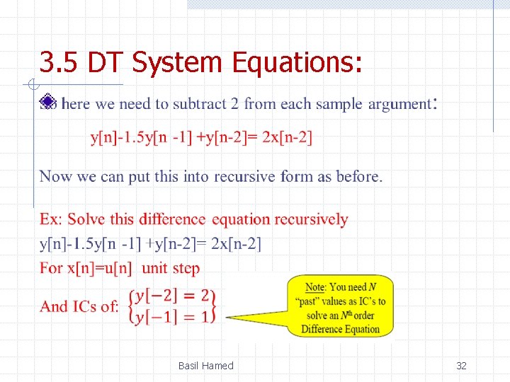
![3. 5 DT System Equations: Recursive Form: y[n]=1. 5 y[n -1] -y[n-2]+ 2 x[n-2] 3. 5 DT System Equations: Recursive Form: y[n]=1. 5 y[n -1] -y[n-2]+ 2 x[n-2]](https://slidetodoc.com/presentation_image_h2/3f9313562ab36b47b73feb4ff5439580/image-33.jpg)
![3. 5 DT System Equations: Ex 3. 9 P. 273 y[n+2]-y[n +1] +0. 24 3. 5 DT System Equations: Ex 3. 9 P. 273 y[n+2]-y[n +1] +0. 24](https://slidetodoc.com/presentation_image_h2/3f9313562ab36b47b73feb4ff5439580/image-34.jpg)
![3. 8 System Response to External Input: (Zero State Response) Step 2: Flip x[k] 3. 8 System Response to External Input: (Zero State Response) Step 2: Flip x[k]](https://slidetodoc.com/presentation_image_h2/3f9313562ab36b47b73feb4ff5439580/image-47.jpg)
![3. 8 System Response to External Input: (Zero State Response) EX: given x[n], and 3. 8 System Response to External Input: (Zero State Response) EX: given x[n], and](https://slidetodoc.com/presentation_image_h2/3f9313562ab36b47b73feb4ff5439580/image-55.jpg)
![3. 8 System Response to External Input: (Zero State Response) y[n]={1, 2, -3, 1, 3. 8 System Response to External Input: (Zero State Response) y[n]={1, 2, -3, 1,](https://slidetodoc.com/presentation_image_h2/3f9313562ab36b47b73feb4ff5439580/image-56.jpg)
- Slides: 63

Signal & Linear system Chapter 3 Time Domain Analysis of DT System Basil Hamed

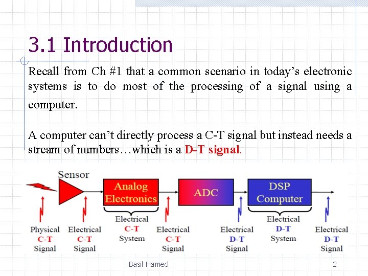
3. 1 Introduction Recall from Ch #1 that a common scenario in today’s electronic systems is to do most of the processing of a signal using a computer. A computer can’t directly process a C-T signal but instead needs a stream of numbers…which is a D-T signal. Basil Hamed 2

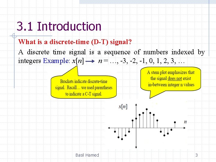
3. 1 Introduction What is a discrete-time (D-T) signal? A discrete time signal is a sequence of numbers indexed by integers Example: x[n] n = …, -3, -2, -1, 0, 1, 2, 3, … Basil Hamed 3

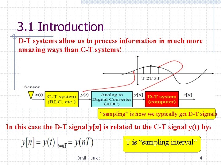
3. 1 Introduction D-T systems allow us to process information in much more amazing ways than C-T systems! “sampling” is how we typically get D-T signals In this case the D-T signal y[n] is related to the C-T signal y(t) by: T is “sampling interval” Basil Hamed 4

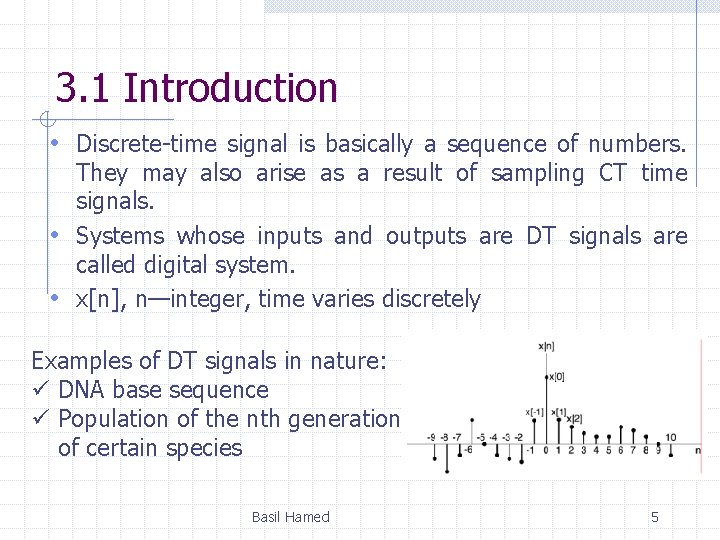
3. 1 Introduction • Discrete-time signal is basically a sequence of numbers. They may also arise as a result of sampling CT time signals. • Systems whose inputs and outputs are DT signals are called digital system. • x[n], n—integer, time varies discretely Examples of DT signals in nature: ü DNA base sequence ü Population of the nth generation of certain species Basil Hamed 5

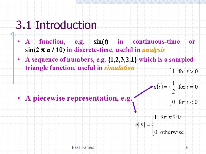
3. 1 Introduction • A function, e. g. sin(t) in continuous-time or sin(2 p n / 10) in discrete-time, useful in analysis • A sequence of numbers, e. g. {1, 2, 3, 2, 1} which is a sampled triangle function, useful in simulation • A piecewise representation, e. g. Basil Hamed 6

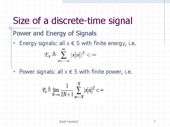
Size of a discrete-time signal Power and Energy of Signals • Energy signals: all x ϵ S with finite energy, i. e. • Power signals: all x ϵ S with finite power, i. e. Basil Hamed 7

3. 2 Useful Signal Operations Three possible time transformations: • Time Shifting • Time Scaling • Time Reversal Basil Hamed 8

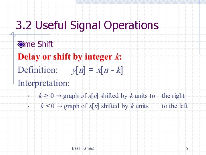
3. 2 Useful Signal Operations Basil Hamed 9
![3 2 Useful Signal Operations Time Shift Signal xn 1 represents instant shifted 3. 2 Useful Signal Operations Time Shift Signal x[n ± 1] represents instant shifted](https://slidetodoc.com/presentation_image_h2/3f9313562ab36b47b73feb4ff5439580/image-10.jpg)
3. 2 Useful Signal Operations Time Shift Signal x[n ± 1] represents instant shifted version of x[n] Find f[k-5] Basil Hamed 10

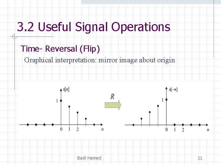
3. 2 Useful Signal Operations Time- Reversal (Flip) Graphical interpretation: mirror image about origin Basil Hamed 11
![3 2 Useful Signal Operations Time Reversal Flip Signal xn represents flip version of 3. 2 Useful Signal Operations Time- Reversal (Flip) Signal x[-n] represents flip version of](https://slidetodoc.com/presentation_image_h2/3f9313562ab36b47b73feb4ff5439580/image-12.jpg)
3. 2 Useful Signal Operations Time- Reversal (Flip) Signal x[-n] represents flip version of x[n] Find f[-k] Basil Hamed 12
![3 2 Useful Signal Operations Timescale Find f2 k fk2 Basil Hamed 13 3. 2 Useful Signal Operations Time-scale Find f[2 k], f[k/2] Basil Hamed 13](https://slidetodoc.com/presentation_image_h2/3f9313562ab36b47b73feb4ff5439580/image-13.jpg)
3. 2 Useful Signal Operations Time-scale Find f[2 k], f[k/2] Basil Hamed 13

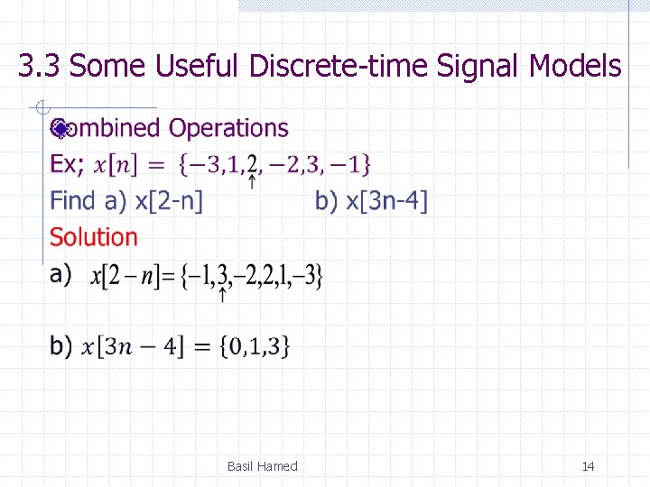
3. 3 Some Useful Discrete-time Signal Models Basil Hamed 14

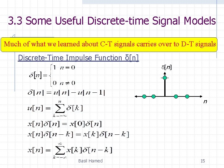
3. 3 Some Useful Discrete-time Signal Models Much of what we learned about C-T signals carries over to D-T signals Discrete-Time Impulse Function δ[n] n Basil Hamed 15
![3 3 Some Useful Discretetime Signal Models DiscreteTime Unit Step Function un unk Basil 3. 3 Some Useful Discrete-time Signal Models Discrete-Time Unit Step Function u[n] u[n-k]= Basil](https://slidetodoc.com/presentation_image_h2/3f9313562ab36b47b73feb4ff5439580/image-16.jpg)
3. 3 Some Useful Discrete-time Signal Models Discrete-Time Unit Step Function u[n] u[n-k]= Basil Hamed 16
![3 3 Some Useful Discretetime Signal Models DiscreteTime Unit ramp Function rn Basil Hamed 3. 3 Some Useful Discrete-time Signal Models Discrete-Time Unit ramp Function r[n]= Basil Hamed](https://slidetodoc.com/presentation_image_h2/3f9313562ab36b47b73feb4ff5439580/image-17.jpg)
3. 3 Some Useful Discrete-time Signal Models Discrete-Time Unit ramp Function r[n]= Basil Hamed 17
![3 3 Some Useful Discretetime Signal Models DT Sinusoids XnAcos Ω n θ Use 3. 3 Some Useful Discrete-time Signal Models D-T Sinusoids X[n]=Acos (Ω n+ θ) Use](https://slidetodoc.com/presentation_image_h2/3f9313562ab36b47b73feb4ff5439580/image-18.jpg)
3. 3 Some Useful Discrete-time Signal Models D-T Sinusoids X[n]=Acos (Ω n+ θ) Use “upper case omega” for frequency of D-T sinusoids What is the unit for Ω? Ωn + θ must be in radians ⇒Ωn in radians Ω is “how many radians jump for each sample” Ω is in radians/sample Basil Hamed 18

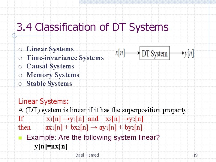
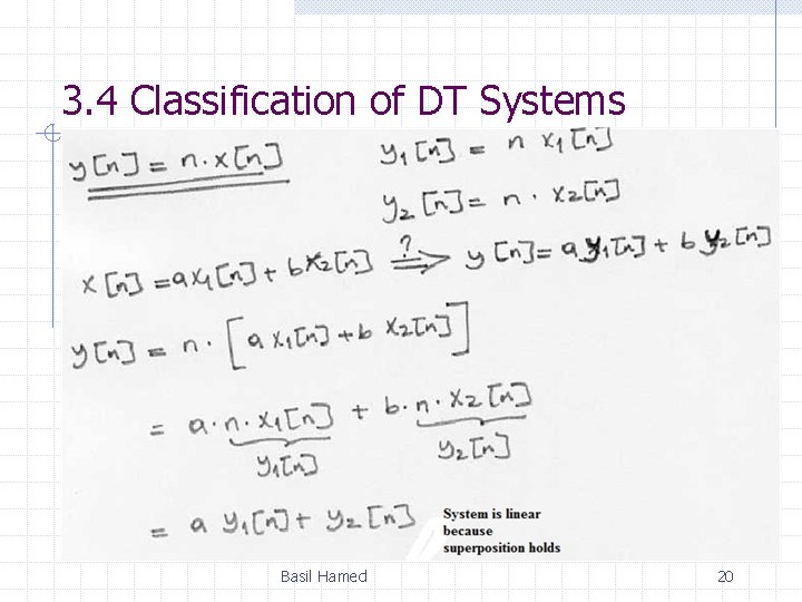
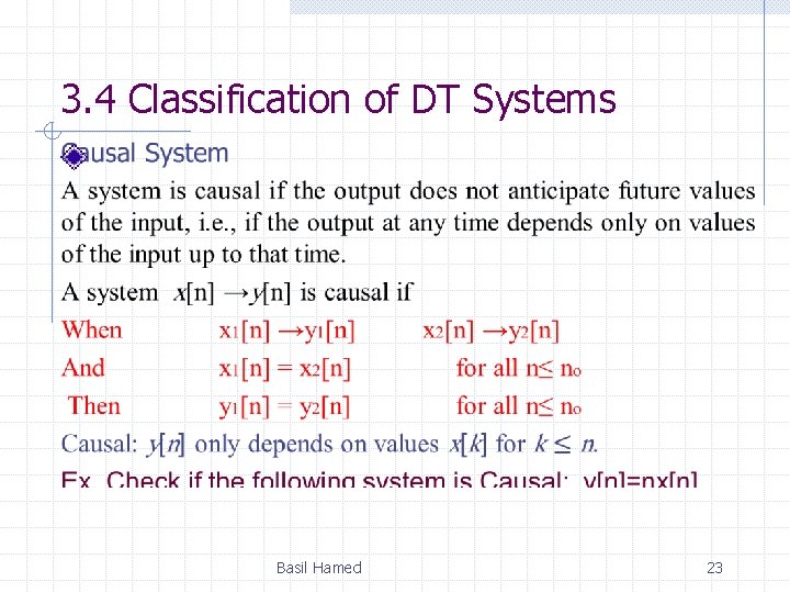
3. 4 Classification of DT Systems o o o Linear Systems Time-invariance Systems Causal Systems Memory Systems Stable Systems Linear Systems: A (DT) system is linear if it has the superposition property: If x 1[n] →y 1[n] and x 2[n] →y 2[n] then ax 1[n] + bx 2[n] → ay 1[n] + by 2[n] n Example: Are the following system linear? y[n]=nx[n] Basil Hamed 19

3. 4 Classification of DT Systems Basil Hamed 20

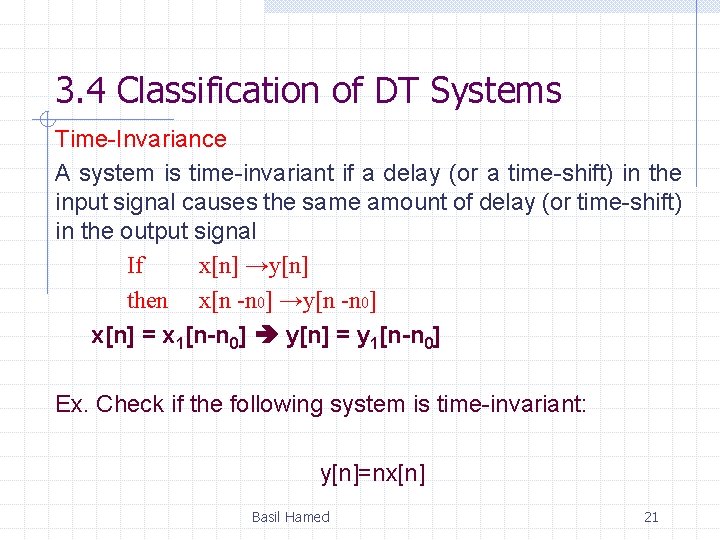
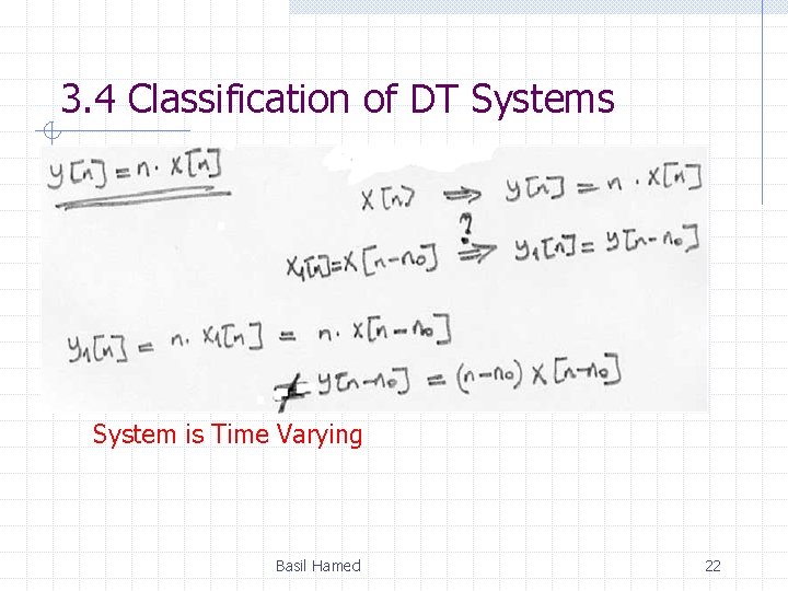
3. 4 Classification of DT Systems Time-Invariance A system is time-invariant if a delay (or a time-shift) in the input signal causes the same amount of delay (or time-shift) in the output signal If x[n] →y[n] then x[n -n 0] →y[n -n 0] x[n] = x 1[n-n 0] y[n] = y 1[n-n 0] Ex. Check if the following system is time-invariant: y[n]=nx[n] Basil Hamed 21

3. 4 Classification of DT Systems System is Time Varying Basil Hamed 22

3. 4 Classification of DT Systems Basil Hamed 23

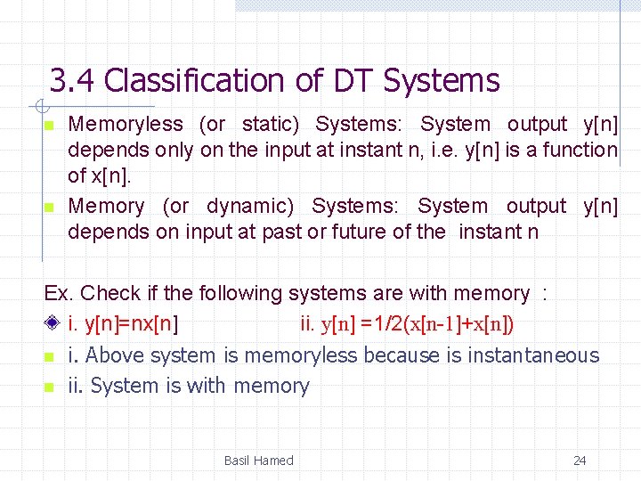
3. 4 Classification of DT Systems n n Memoryless (or static) Systems: System output y[n] depends only on the input at instant n, i. e. y[n] is a function of x[n]. Memory (or dynamic) Systems: System output y[n] depends on input at past or future of the instant n Ex. Check if the following systems are with memory : i. y[n]=nx[n] ii. y[n] =1/2(x[n-1]+x[n]) n i. Above system is memoryless because is instantaneous n ii. System is with memory Basil Hamed 24

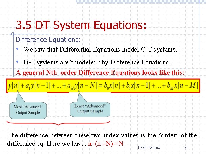
3. 5 DT System Equations: Difference Equations: • We saw that Differential Equations model C-T systems… • D-T systems are “modeled” by Difference Equations. A general Nth order Difference Equations looks like this: The difference between these two index values is the “order” of the difference eq. Here we have: n–(n –N) =N Basil Hamed 25

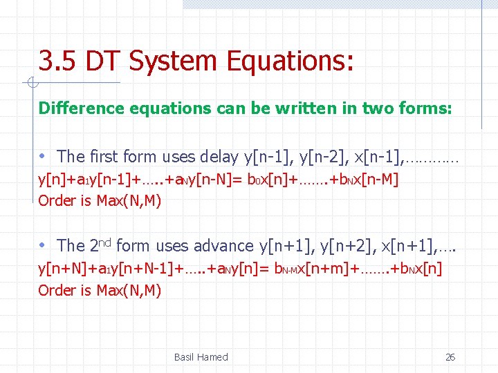
3. 5 DT System Equations: Difference equations can be written in two forms: • The first form uses delay y[n-1], y[n-2], x[n-1], ………… y[n]+a 1 y[n-1]+…. . +a. Ny[n-N]= b 0 x[n]+……. +b. Nx[n-M] Order is Max(N, M) • The 2 nd form uses advance y[n+1], y[n+2], x[n+1], …. y[n+N]+a 1 y[n+N-1]+…. . +a. Ny[n]= b. N-Mx[n+m]+……. +b. Nx[n] Order is Max(N, M) Basil Hamed 26

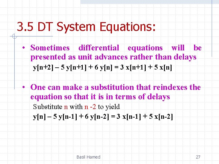
3. 5 DT System Equations: • Sometimes differential equations will be presented as unit advances rather than delays y[n+2] – 5 y[n+1] + 6 y[n] = 3 x[n+1] + 5 x[n] • One can make a substitution that reindexes the equation so that it is in terms of delays Substitute n with n -2 to yield y[n] – 5 y[n-1] + 6 y[n-2] = 3 x[n-1] + 5 x[n-2] Basil Hamed 27

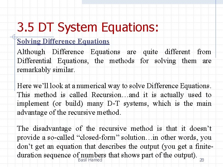
3. 5 DT System Equations: Solving Difference Equations Although Difference Equations are quite different from Differential Equations, the methods for solving them are remarkably similar. Here we’ll look at a numerical way to solve Difference Equations. This method is called Recursion…and it is actually used to implement (or build) many D-T systems, which is the main advantage of the recursive method. The disadvantage of the recursive method is that it doesn’t provide a so-called “closed-form” solution…in other words, you don’t get an equation that describes the output (you get a finiteduration sequence of numbers that shows part of the output). Basil Hamed 28

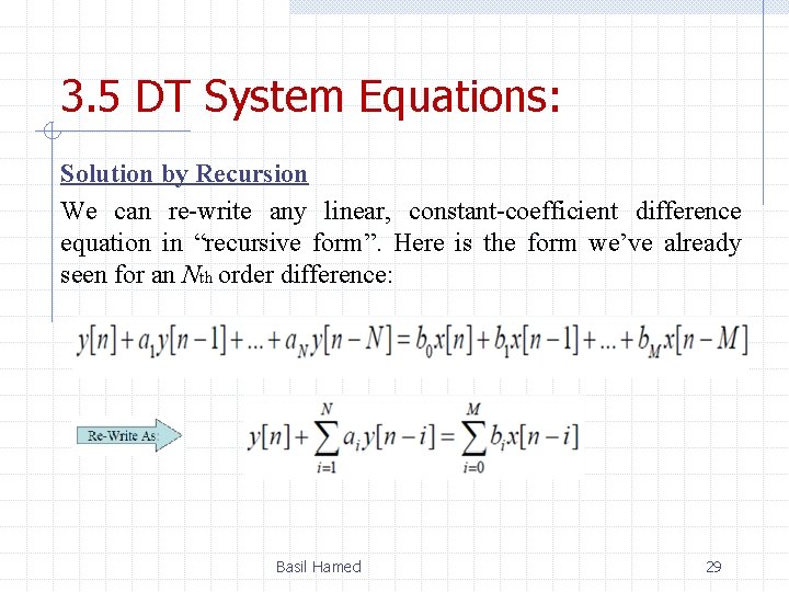
3. 5 DT System Equations: Solution by Recursion We can re-write any linear, constant-coefficient difference equation in “recursive form”. Here is the form we’ve already seen for an Nth order difference: Basil Hamed 29
![3 5 DT System Equations Nowisolating the yn term gives the Recursive Form current 3. 5 DT System Equations: Now…isolating the y[n] term gives the “Recursive Form”: “current”](https://slidetodoc.com/presentation_image_h2/3f9313562ab36b47b73feb4ff5439580/image-30.jpg)
3. 5 DT System Equations: Now…isolating the y[n] term gives the “Recursive Form”: “current” Output value to be computed Some “past” output values, with values already known Basil Hamed current & past input values already “received” 30

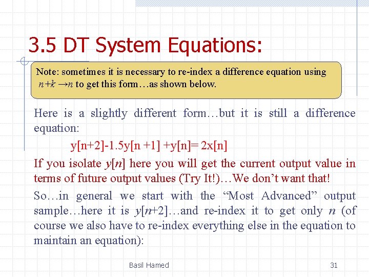
3. 5 DT System Equations: Note: sometimes it is necessary to re-index a difference equation using n+k →n to get this form…as shown below. Here is a slightly different form…but it is still a difference equation: y[n+2]-1. 5 y[n +1] +y[n]= 2 x[n] If you isolate y[n] here you will get the current output value in terms of future output values (Try It!)…We don’t want that! So…in general we start with the “Most Advanced” output sample…here it is y[n+2]…and re-index it to get only n (of course we also have to re-index everything else in the equation to maintain an equation): Basil Hamed 31

3. 5 DT System Equations: Basil Hamed 32
![3 5 DT System Equations Recursive Form yn1 5 yn 1 yn2 2 xn2 3. 5 DT System Equations: Recursive Form: y[n]=1. 5 y[n -1] -y[n-2]+ 2 x[n-2]](https://slidetodoc.com/presentation_image_h2/3f9313562ab36b47b73feb4ff5439580/image-33.jpg)
3. 5 DT System Equations: Recursive Form: y[n]=1. 5 y[n -1] -y[n-2]+ 2 x[n-2] Basil Hamed 33
![3 5 DT System Equations Ex 3 9 P 273 yn2yn 1 0 24 3. 5 DT System Equations: Ex 3. 9 P. 273 y[n+2]-y[n +1] +0. 24](https://slidetodoc.com/presentation_image_h2/3f9313562ab36b47b73feb4ff5439580/image-34.jpg)
3. 5 DT System Equations: Ex 3. 9 P. 273 y[n+2]-y[n +1] +0. 24 y[n]= x[n+2]-2 x[n+1] y[-1]=2, y[-2]=1, and causal input x[n]=n Solution y[n]=y[n -1] -0. 24 y[n-2]+ x[n]-2 x[n-1] y[0]=y[-1] -0. 24 y[-2]+ x[0]-2 x[-1]= 2 -0. 24= 1. 76 y[1]=y[0] -0. 24 y[-1]+ x[1]-2 x[0]= 1. 76 – 0. 24(2)+ 1 - 0= 2. 28 : : Basil Hamed 34

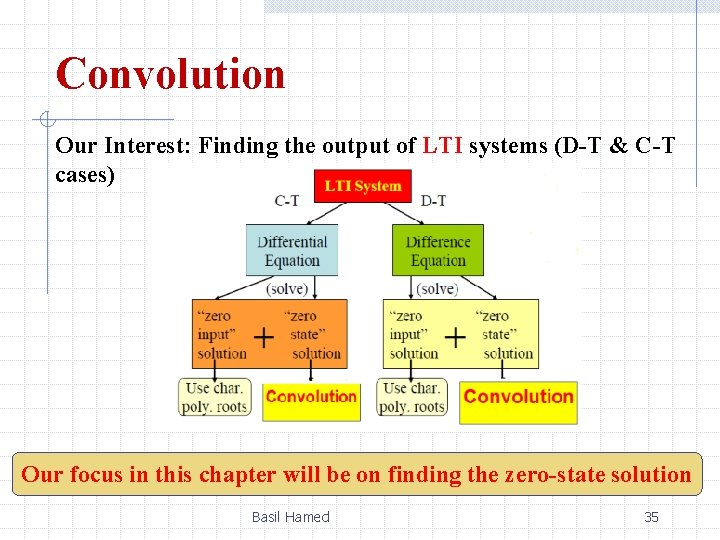
Convolution Our Interest: Finding the output of LTI systems (D-T & C-T cases) Our focus in this chapter will be on finding the zero-state solution Basil Hamed 35

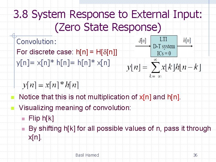
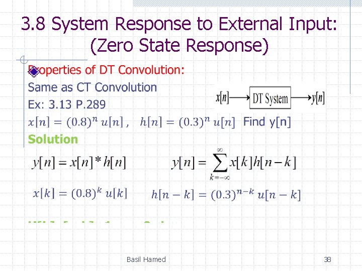
3. 8 System Response to External Input: (Zero State Response) Convolution: For discrete case: h[n] = H[ [n]] y[n]= x[n]* h[n]= h[n]* x[n] n Notice that this is not multiplication of x[n] and h[n]. n Visualizing meaning of convolution: n Flip h[k] n By shifting h[k] for all possible values of n, pass it through x[n]. Basil Hamed 36

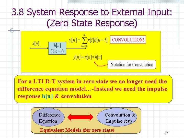
3. 8 System Response to External Input: (Zero State Response) For a LTI D-T system in zero state we no longer need the difference equation model…-Instead we need the impulse response h[n] & convolution Difference Equation Convolution & Impulse resp Equivalent Basil Models Hamed(for zero state) 37

3. 8 System Response to External Input: (Zero State Response) Basil Hamed 38

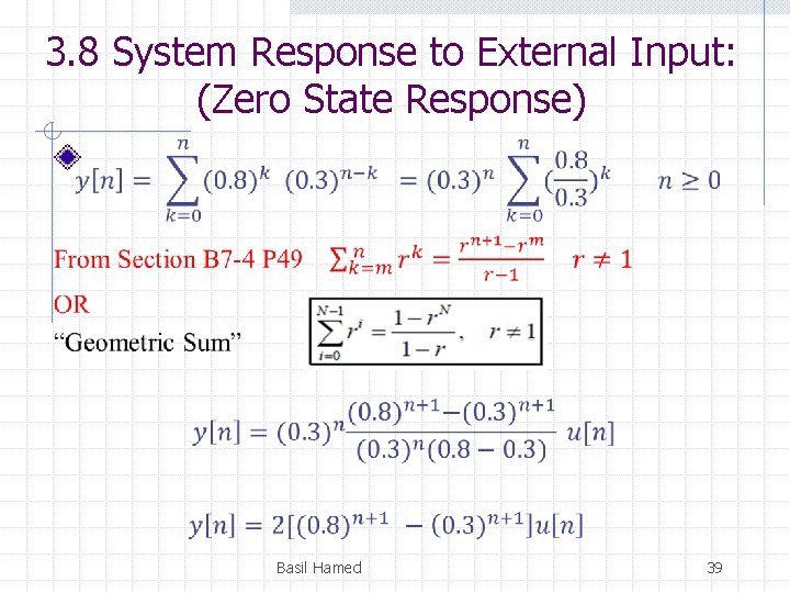
3. 8 System Response to External Input: (Zero State Response) Basil Hamed 39

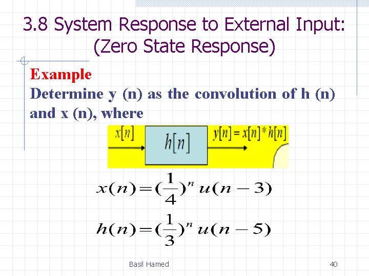
3. 8 System Response to External Input: (Zero State Response) Example Determine y (n) as the convolution of h (n) and x (n), where Basil Hamed 40

3. 8 System Response to External Input: (Zero State Response) Basil Hamed 41

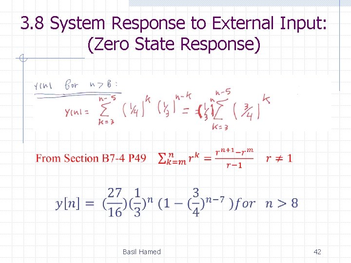
3. 8 System Response to External Input: (Zero State Response) Basil Hamed 42

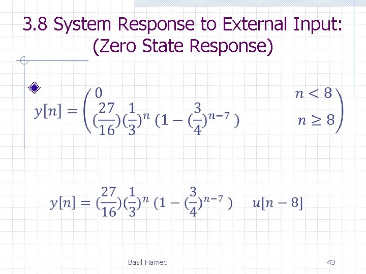
3. 8 System Response to External Input: (Zero State Response) Basil Hamed 43

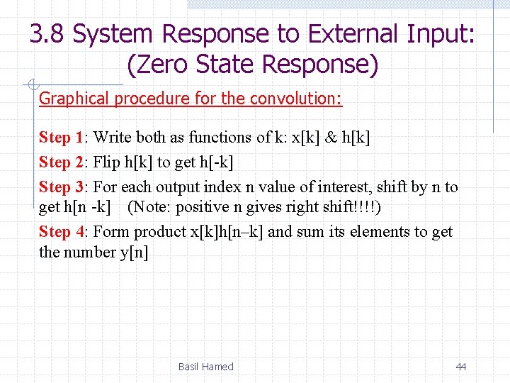
3. 8 System Response to External Input: (Zero State Response) Graphical procedure for the convolution: Step 1: Write both as functions of k: x[k] & h[k] Step 2: Flip h[k] to get h[-k] Step 3: For each output index n value of interest, shift by n to get h[n -k] (Note: positive n gives right shift!!!!) Step 4: Form product x[k]h[n–k] and sum its elements to get the number y[n] Basil Hamed 44

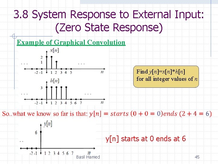
3. 8 System Response to External Input: (Zero State Response) Example of Graphical Convolution Find y[n]=x[n]*h[n] for all integer values of n y[n] starts at 0 ends at 6 Basil Hamed 45

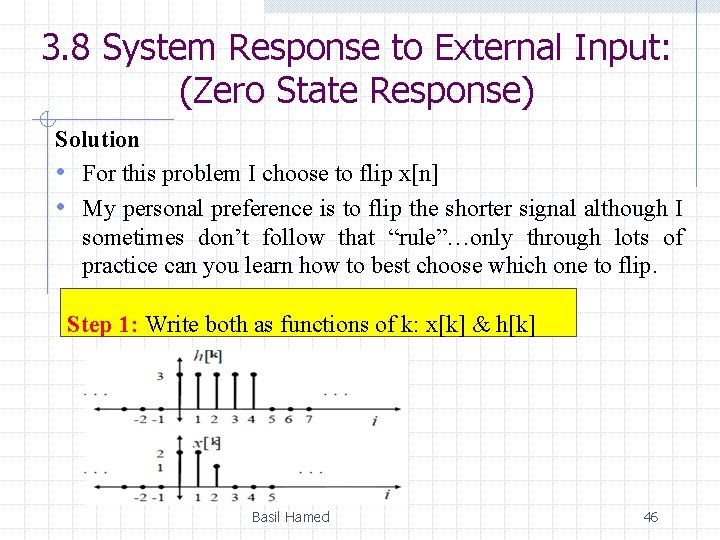
3. 8 System Response to External Input: (Zero State Response) Solution • For this problem I choose to flip x[n] • My personal preference is to flip the shorter signal although I sometimes don’t follow that “rule”…only through lots of practice can you learn how to best choose which one to flip. Step 1: Write both as functions of k: x[k] & h[k] Basil Hamed 46
![3 8 System Response to External Input Zero State Response Step 2 Flip xk 3. 8 System Response to External Input: (Zero State Response) Step 2: Flip x[k]](https://slidetodoc.com/presentation_image_h2/3f9313562ab36b47b73feb4ff5439580/image-47.jpg)
3. 8 System Response to External Input: (Zero State Response) Step 2: Flip x[k] to get x[-k] “Commutativity” says we can flip either x[k] or h[k] and get the same answer… Here I flipped x[k] Basil Hamed 47

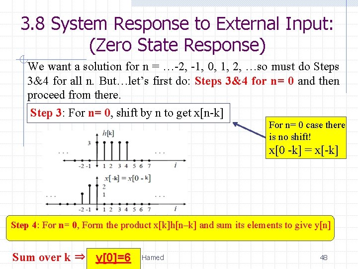
3. 8 System Response to External Input: (Zero State Response) We want a solution for n = …-2, -1, 0, 1, 2, …so must do Steps 3&4 for all n. But…let’s first do: Steps 3&4 for n= 0 and then proceed from there. Step 3: For n= 0, shift by n to get x[n-k] For n= 0 case there is no shift! x[0 -k] = x[-k] Step 4: For n= 0, Form the product x[k]h[n–k] and sum its elements to give y[n] Sum over k ⇒ y[0]=6 Basil Hamed 48

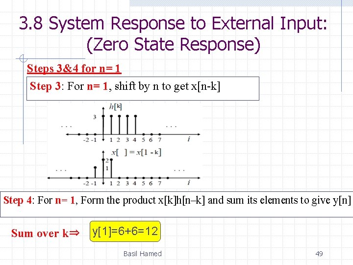
3. 8 System Response to External Input: (Zero State Response) Steps 3&4 for n= 1 Step 3: For n= 1, shift by n to get x[n-k] Step 4: For n= 1, Form the product x[k]h[n–k] and sum its elements to give y[n] Sum over k⇒ y[1]=6+6=12 Basil Hamed 49

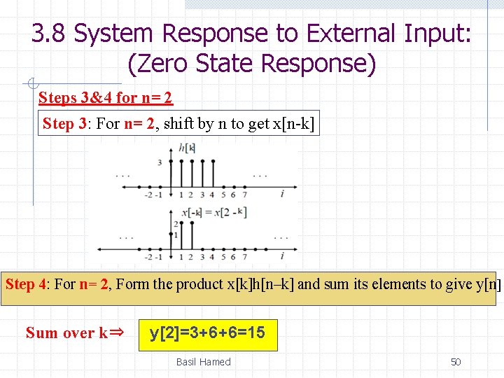
3. 8 System Response to External Input: (Zero State Response) Steps 3&4 for n= 2 Step 3: For n= 2, shift by n to get x[n-k] Step 4: For n= 2, Form the product x[k]h[n–k] and sum its elements to give y[n] Sum over k⇒ y[2]=3+6+6=15 Basil Hamed 50

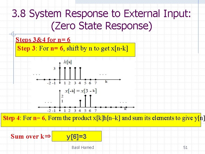
3. 8 System Response to External Input: (Zero State Response) Steps 3&4 for n= 6 Step 3: For n= 6, shift by n to get x[n-k] Step 4: For n= 6, Form the product x[k]h[n–k] and sum its elements to give y[n] Sum over k⇒ y[6]=3 Basil Hamed 51

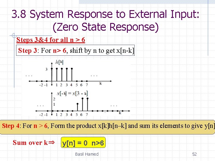
3. 8 System Response to External Input: (Zero State Response) Steps 3&4 for all n > 6 Step 3: For n> 6, shift by n to get x[n-k] Step 4: For n > 6, Form the product x[k]h[n–k] and sum its elements to give y[n] Sum over k⇒ y[n] = 0 n>6 Basil Hamed 52

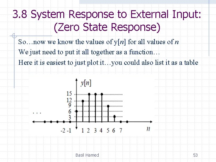
3. 8 System Response to External Input: (Zero State Response) So…now we know the values of y[n] for all values of n We just need to put it all together as a function… Here it is easiest to just plot it…you could also list it as a table Basil Hamed 53

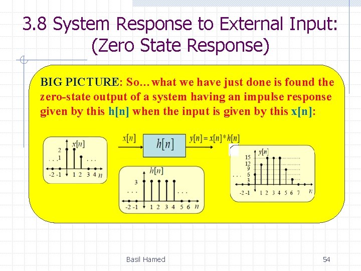
3. 8 System Response to External Input: (Zero State Response) BIG PICTURE: So…what we have just done is found the zero-state output of a system having an impulse response given by this h[n] when the input is given by this x[n]: Basil Hamed 54
![3 8 System Response to External Input Zero State Response EX given xn and 3. 8 System Response to External Input: (Zero State Response) EX: given x[n], and](https://slidetodoc.com/presentation_image_h2/3f9313562ab36b47b73feb4ff5439580/image-55.jpg)
3. 8 System Response to External Input: (Zero State Response) EX: given x[n], and h[n], find y[n] Basil Hamed 55
![3 8 System Response to External Input Zero State Response yn1 2 3 1 3. 8 System Response to External Input: (Zero State Response) y[n]={1, 2, -3, 1,](https://slidetodoc.com/presentation_image_h2/3f9313562ab36b47b73feb4ff5439580/image-56.jpg)
3. 8 System Response to External Input: (Zero State Response) y[n]={1, 2, -3, 1, 1} Basil Hamed 56

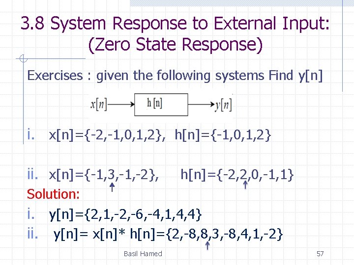
3. 8 System Response to External Input: (Zero State Response) Exercises : given the following systems Find y[n] i. x[n]={-2, -1, 0, 1, 2}, h[n]={-1, 0, 1, 2} ii. x[n]={-1, 3, -1, -2}, h[n]={-2, 2, 0, -1, 1} Solution: i. y[n]={2, 1, -2, -6, -4, 1, 4, 4} ii. y[n]= x[n]* h[n]={2, -8, 8, 3, -8, 4, 1, -2} Basil Hamed 57

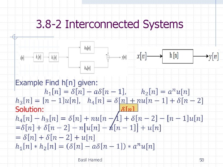
3. 8 -2 Interconnected Systems Basil Hamed 58

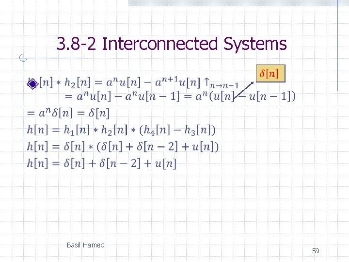
3. 8 -2 Interconnected Systems Basil Hamed 59

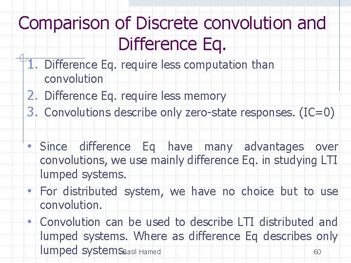
Comparison of Discrete convolution and Difference Eq. 1. Difference Eq. require less computation than convolution 2. Difference Eq. require less memory 3. Convolutions describe only zero-state responses. (IC=0) • Since difference Eq have many advantages over convolutions, we use mainly difference Eq. in studying LTI lumped systems. • For distributed system, we have no choice but to use convolution. • Convolution can be used to describe LTI distributed and lumped systems. Where as difference Eq describes only 60 lumped systems. Basil Hamed

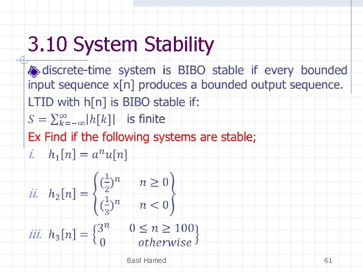
3. 10 System Stability Basil Hamed 61

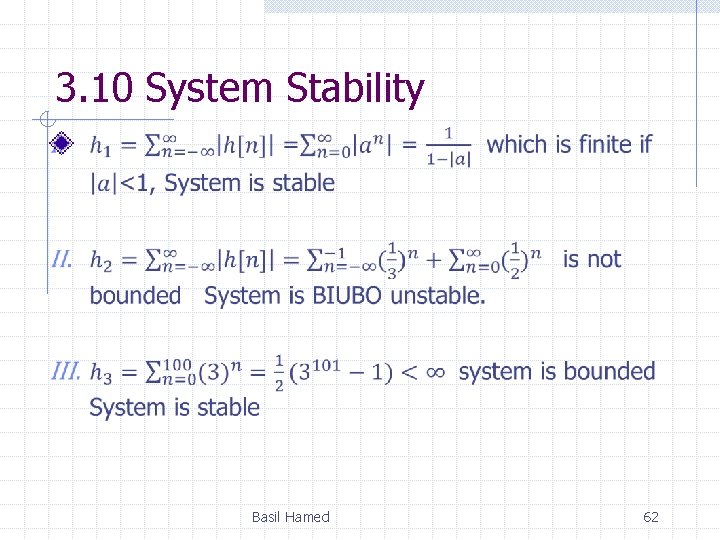
3. 10 System Stability Basil Hamed 62

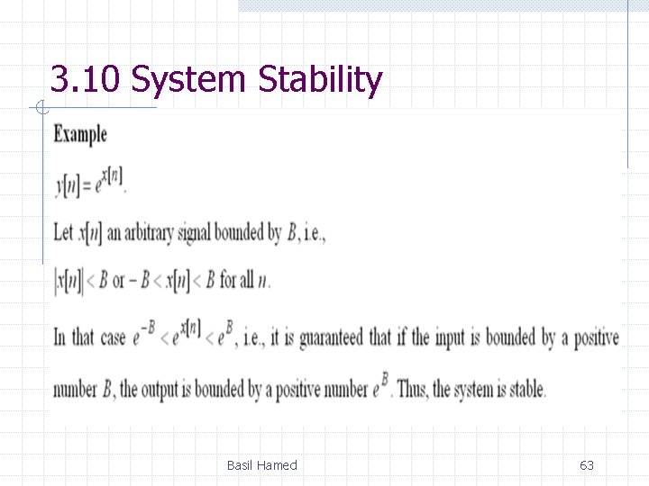
3. 10 System Stability Basil Hamed 63