CHAPTER 2 Time Domain Representation of Linear Time

2. 0 Time Domain Representation of Linear Time Invariant (LTI) System. 2. 1 2.

2. 1 Introduction. Learning Outcome: Examine several methods for describing the relationship between the

2. 2 LTI System Properties. þ If we know the response of the LTI

2. 3 Convolution Sum. þ x[n] is a signal as a weighted sum of

Cont’d… Figure 2. 1: Graphical example illustrating the representation of a signal x[n] as

Cont’d… Steps for Convolution Computation. Step 1: Plot x and h versus k since

Example 2. 1: Convolution Sum. For the figure below, compute the convolution, y[n]. Figure

Solution: ý. Figure 2. 2 b: The decomposition of the input x[n] into a

2. 3. 1 Convolution Sum Evaluation Procedure. þ An alternative approach to evaluating the

Slides: 12

Download presentation

CHAPTER 2 Time Domain Representation of Linear Time Invariant (LTI). EKT 230 1

2. 0 Time Domain Representation of Linear Time Invariant (LTI) System. 2. 1 2. 2 2. 3 Introduction. LTI System Properties. Convolution Sum. 2

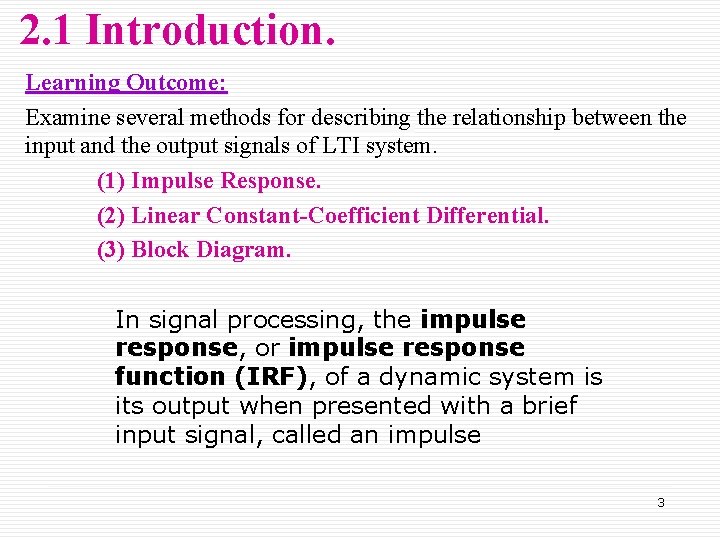
2. 1 Introduction. Learning Outcome: Examine several methods for describing the relationship between the input and the output signals of LTI system. (1) Impulse Response. (2) Linear Constant-Coefficient Differential. (3) Block Diagram. In signal processing, the impulse response, or impulse response function (IRF), of a dynamic system is its output when presented with a brief input signal, called an impulse 3

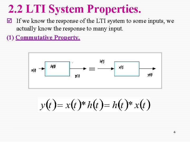
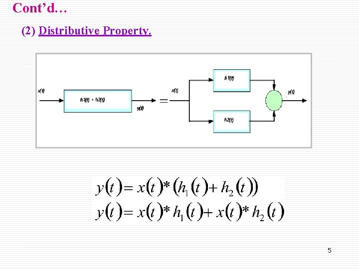
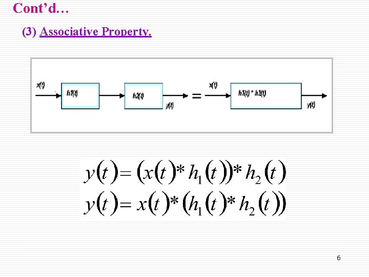
2. 2 LTI System Properties. þ If we know the response of the LTI system to some inputs, we actually know the response to many input. (1) Commutative Property. 4

Cont’d… (2) Distributive Property. 5

Cont’d… (3) Associative Property. 6

2. 3 Convolution Sum. þ x[n] is a signal as a weighted sum of basis function; time-shift version of the unit impulse signal. x[k] represents a specific value of the signal x[n] at time k. þ The output of the LTI system y[n] is given by a weighted sum of time-shifted impulse response. h[n] is the impulse response of LTI system H. þ The convolution of two discrete-time signals y[n ] and h[n] is denoted as 7

Cont’d… Figure 2. 1: Graphical example illustrating the representation of a signal x[n] as a weighted sum of time-shifted impulses. 8

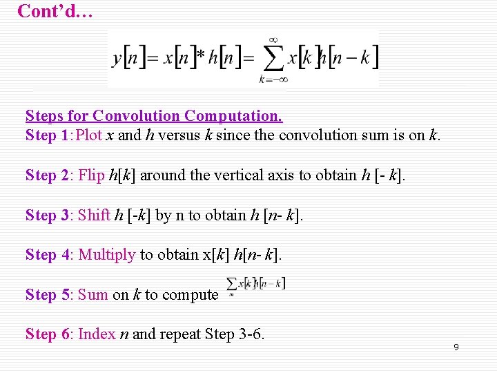
Cont’d… Steps for Convolution Computation. Step 1: Plot x and h versus k since the convolution sum is on k. 1 Step 2: 2 Flip h[k] around the vertical axis to obtain h [- k]. Step 3: 3 Shift h [-k] by n to obtain h [n- k]. Step 4: 4 Multiply to obtain x[k] h[n- k]. Step 5: 5 Sum on k to compute Step 6: 6 Index n and repeat Step 3 -6. 9

Example 2. 1: Convolution Sum. For the figure below, compute the convolution, y[n]. Figure 2. 2 a: Illustration of the convolution sum. (a) LTI system with impulse response h[n] and input x[n], producing y[n] and yet to be determined. 10

Solution: ý. Figure 2. 2 b: The decomposition of the input x[n] into a weighted sum of timeshifted impulses results in an output y[n] given by a weighted sum of time 11 shifted impulse responses.

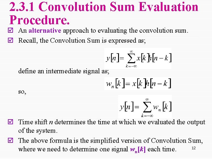
2. 3. 1 Convolution Sum Evaluation Procedure. þ An alternative approach to evaluating the convolution sum. þ Recall, the Convolution Sum is expressed as; define an intermediate signal as; so, þ Time shift n determines the time at which we evaluated the output of the system. þ The above formula is the simplified version of Convolution Sum, 12 where we need to determine one signal wn[k] each time.