Queuing Theory Overview Introduction MM1 MMsK MMs with

Queuing Theory

Overview • Introduction • M/M/1 • M/M/s/K • M/M/s with finite calling population 040669 || WS 2008 || Dr. Verena Schmid || PR KFK PM/SCM/TL Praktikum Simulation I

Introduction • queuing theory? –mathematical study of queues and waiting lines • waiting line? –current demand for service exceeds current capacity to provide service • how much service to provide? –providing too much is costly –but: excessive waiting is costly –impossible to predict accurately when units arrive to seek service and/or how much time is required to provide service 040669 || WS 2008 || Dr. Verena Schmid || PR KFK PM/SCM/TL Praktikum Simulation I

Introduction • queuing theory –does not solve problems related to stochastics directly –provides useful information required by decision makers • average # in waiting line / system • average waiting time • average time in system • utilization rate 040669 || WS 2008 || Dr. Verena Schmid || PR KFK PM/SCM/TL Praktikum Simulation I

Basic Queuing Process • input source –customers requiring a service are generated over time • customers –enter queuing system –join a queue • queue discipline –member of queue is selected for service by some rule (f. e. FCFS) • service mechanism –required service is performed for the customer 040669 || WS 2008 || Dr. Verena Schmid || PR KFK PM/SCM/TL Praktikum Simulation I

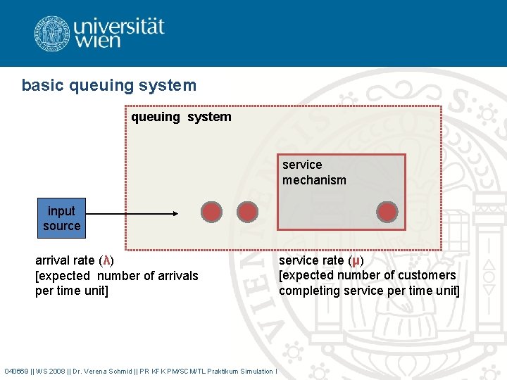
basic queuing system service mechanism input source arrival rate (λ) [expected number of arrivals per time unit] 040669 || WS 2008 || Dr. Verena Schmid || PR KFK PM/SCM/TL Praktikum Simulation I service rate (μ) [expected number of customers completing service per time unit]

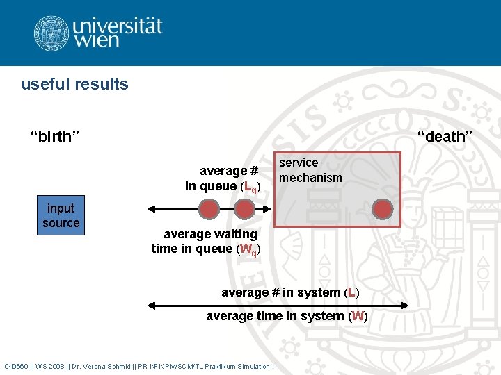
useful results “birth” “death” average # in queue (Lq) input source service mechanism average waiting time in queue (Wq) average # in system (L) average time in system (W) 040669 || WS 2008 || Dr. Verena Schmid || PR KFK PM/SCM/TL Praktikum Simulation I

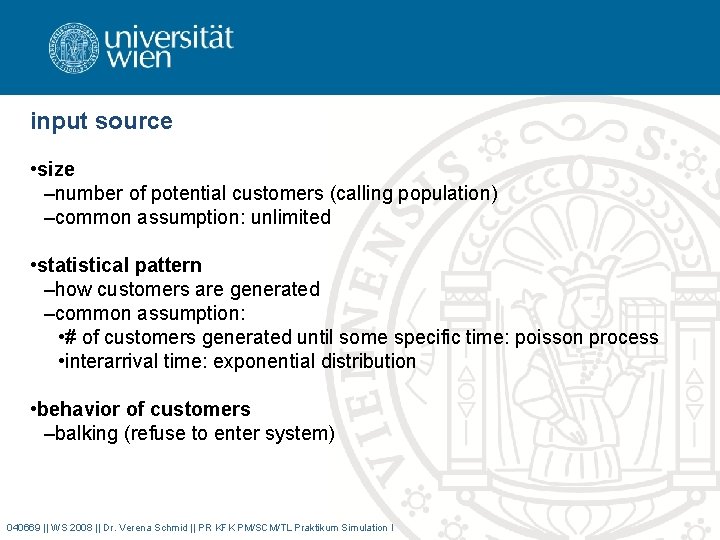
input source • size –number of potential customers (calling population) –common assumption: unlimited • statistical pattern –how customers are generated –common assumption: • # of customers generated until some specific time: poisson process • interarrival time: exponential distribution • behavior of customers –balking (refuse to enter system) 040669 || WS 2008 || Dr. Verena Schmid || PR KFK PM/SCM/TL Praktikum Simulation I

queue • queue capacity –maximum permissible number of customers that can be in queue –finite vs. infinite • queuing discipline –order how members of queue are selected –first-come-first-served –random –priority procedure 040669 || WS 2008 || Dr. Verena Schmid || PR KFK PM/SCM/TL Praktikum Simulation I

service mechanism • one or more service facilities • each of them: one or more parallel service channels (servers) • service time –how long does it take to serve customers? –follows some probability distribution • common: assume same for all servers • exponential distribution • Erlang distribution • break downs? 040669 || WS 2008 || Dr. Verena Schmid || PR KFK PM/SCM/TL Praktikum Simulation I

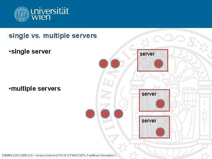
single vs. multiple servers • single server • multiple servers server 040669 || WS 2008 || Dr. Verena Schmid || PR KFK PM/SCM/TL Praktikum Simulation I

remarks • server –not necessarily a single person –could be machine as well • queue –not necessarily a line (waiting room) • Kendall notation: X / Y / s –X distribution of arrivals –Y distribution of service times • M exponential distribution (memoryless) • D deterministic • Ek Erlang distribution • G general distribution –s number of servers 040669 || WS 2008 || Dr. Verena Schmid || PR KFK PM/SCM/TL Praktikum Simulation I

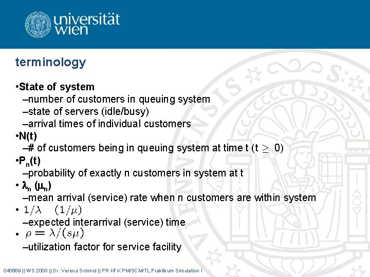
terminology • State of system –number of customers in queuing system –state of servers (idle/busy) –arrival times of individual customers • N(t) –# of customers being in queuing system at time t (t ¸ 0) • Pn(t) –probability of exactly n customers in system at t • n ( n) –mean arrival (service) rate when n customers are within system • –expected interarrival (service) time • –utilization factor for service facility 040669 || WS 2008 || Dr. Verena Schmid || PR KFK PM/SCM/TL Praktikum Simulation I

system status changes over time • at start –depends on initial state and on time already elapsed –system is in a transient condition • after sufficient time elapsed –state of system becomes independent of initial state –system eventually reached a steady-state condition –probability distribution of state of system remains unchanged 040669 || WS 2008 || Dr. Verena Schmid || PR KFK PM/SCM/TL Praktikum Simulation I

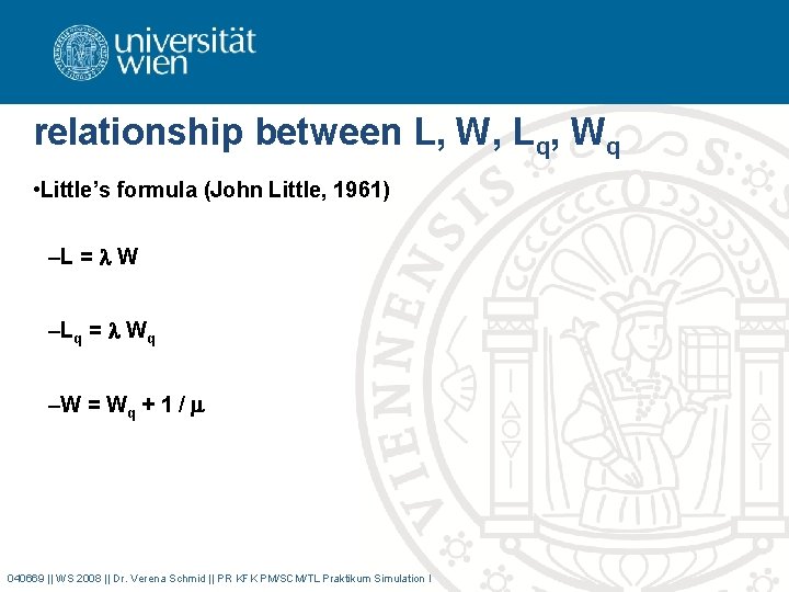
relationship between L, W, Lq, Wq • Little’s formula (John Little, 1961) –L = W –L q = W q –W = W q + 1 / 040669 || WS 2008 || Dr. Verena Schmid || PR KFK PM/SCM/TL Praktikum Simulation I

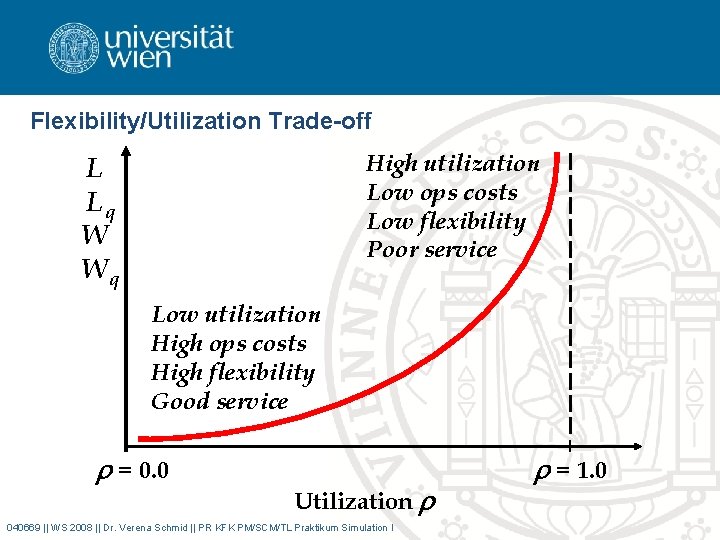
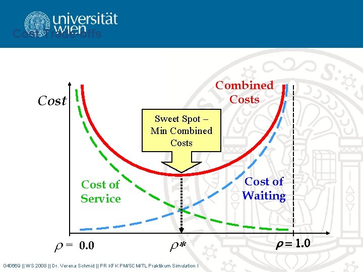
Managerial Implications • Low utilization levels provide –better service levels –greater flexibility –lower waiting costs (e. g. , lost business) • High utilization levels provide –better equipment and employee utilization –fewer idle periods –lower production/service costs • Must trade off benefits of high utilization levels with benefits of flexibility and service 040669 || WS 2008 || Dr. Verena Schmid || PR KFK PM/SCM/TL Praktikum Simulation I

Flexibility/Utilization Trade-off High utilization Low ops costs Low flexibility Poor service L Lq W Wq Low utilization High ops costs High flexibility Good service = 0. 0 Utilization 040669 || WS 2008 || Dr. Verena Schmid || PR KFK PM/SCM/TL Praktikum Simulation I = 1. 0

Cost Trade-offs Combined Costs Cost Sweet Spot – Min Combined Costs Cost of Waiting Cost of Service = 0. 0 * 040669 || WS 2008 || Dr. Verena Schmid || PR KFK PM/SCM/TL Praktikum Simulation I = 1. 0

birth- and death process • describes how N(t) changes as t increases • given N(t) = n, –the current probability distribution of the remaining time until the next birth (arrival) is exponential with parameter n –the current probability distribution of the remaining time until the next death (departure) is exponential with parameter n • random variables are mutually independent • special type of continuous time Markov chain 040669 || WS 2008 || Dr. Verena Schmid || PR KFK PM/SCM/TL Praktikum Simulation I

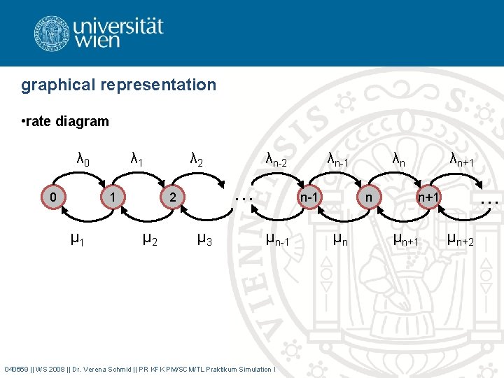
graphical representation • rate diagram λ 0 0 λ 1 1 μ 1 λ 2 … 2 μ 2 λn-2 μ 3 λn-1 μn-1 040669 || WS 2008 || Dr. Verena Schmid || PR KFK PM/SCM/TL Praktikum Simulation I λn n μn λn+1 … n+1 μn+2

rate in = rate out • in equilibrium, the tendency to move out of a certain state must equal the tendency to move towards that state • balance equations for state n 040669 || WS 2008 || Dr. Verena Schmid || PR KFK PM/SCM/TL Praktikum Simulation I

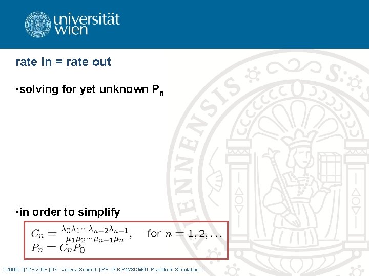
rate in = rate out • solving for yet unknown Pn • in order to simplify 040669 || WS 2008 || Dr. Verena Schmid || PR KFK PM/SCM/TL Praktikum Simulation I

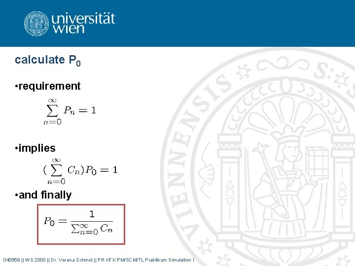
calculate P 0 • requirement • implies • and finally 040669 || WS 2008 || Dr. Verena Schmid || PR KFK PM/SCM/TL Praktikum Simulation I

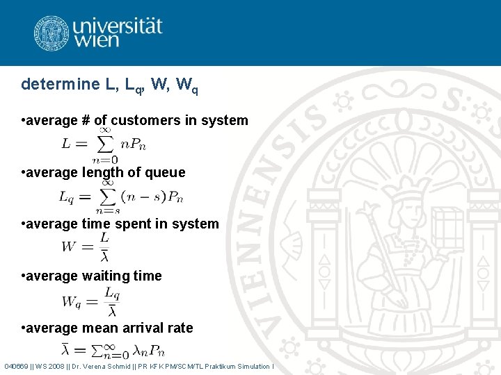
determine L, Lq, W, Wq • average # of customers in system • average length of queue • average time spent in system • average waiting time • average mean arrival rate 040669 || WS 2008 || Dr. Verena Schmid || PR KFK PM/SCM/TL Praktikum Simulation I

M/M/1 single server model

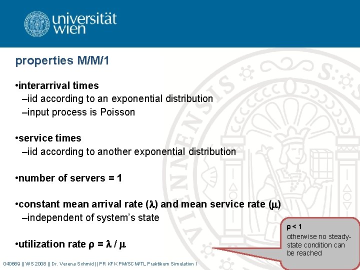
properties M/M/1 • interarrival times –iid according to an exponential distribution –input process is Poisson • service times –iid according to another exponential distribution • number of servers = 1 • constant mean arrival rate ( ) and mean service rate ( ) –independent of system’s state • utilization rate = / 040669 || WS 2008 || Dr. Verena Schmid || PR KFK PM/SCM/TL Praktikum Simulation I <1 otherwise no steadystate condition can be reached

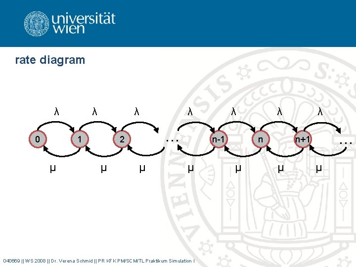
rate diagram λ 0 λ λ 1 μ λ … 2 μ μ λ n-1 μ 040669 || WS 2008 || Dr. Verena Schmid || PR KFK PM/SCM/TL Praktikum Simulation I λ n μ λ … n+1 μ μ

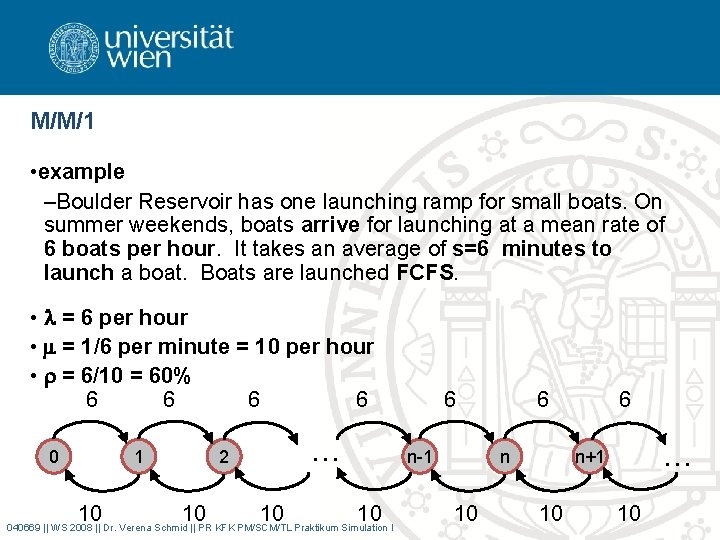
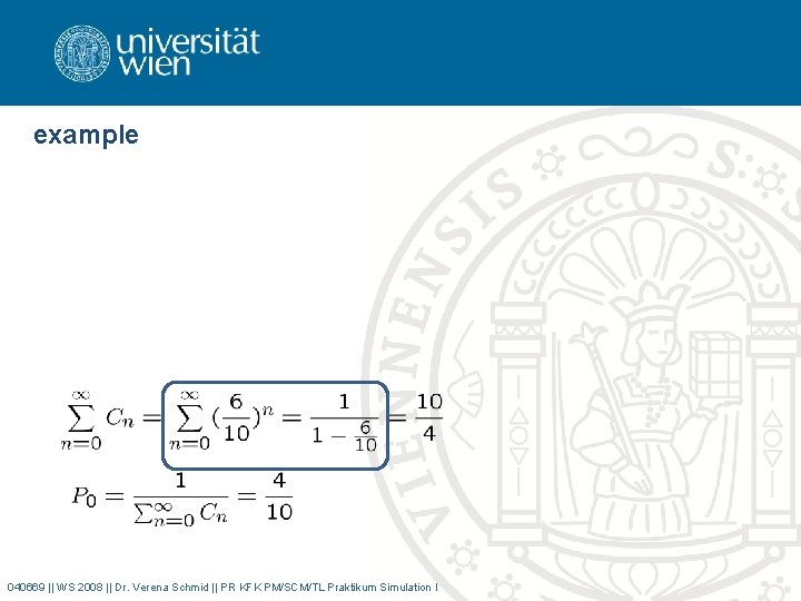
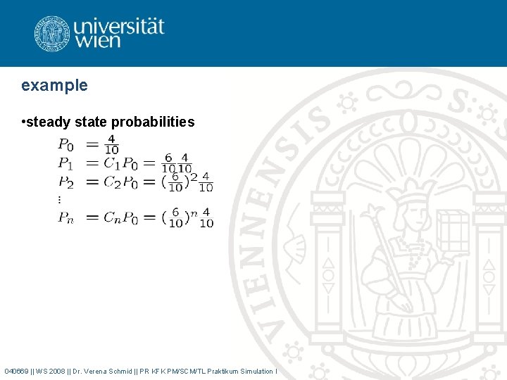
M/M/1 • example –Boulder Reservoir has one launching ramp for small boats. On summer weekends, boats arrive for launching at a mean rate of 6 boats per hour. It takes an average of s=6 minutes to launch a boat. Boats are launched FCFS. • = 6 per hour • = 1/6 per minute = 10 per hour • = 6/10 = 60% 6 6 0 1 10 … 2 10 10 6 n-1 10 040669 || WS 2008 || Dr. Verena Schmid || PR KFK PM/SCM/TL Praktikum Simulation I 6 n 10 6 … n+1 10 10

example 040669 || WS 2008 || Dr. Verena Schmid || PR KFK PM/SCM/TL Praktikum Simulation I

example • steady state probabilities 040669 || WS 2008 || Dr. Verena Schmid || PR KFK PM/SCM/TL Praktikum Simulation I

example • average # in system 040669 || WS 2008 || Dr. Verena Schmid || PR KFK PM/SCM/TL Praktikum Simulation I

formulas for M/M/1 040669 || WS 2008 || Dr. Verena Schmid || PR KFK PM/SCM/TL Praktikum Simulation I

M/M/s multiple server model

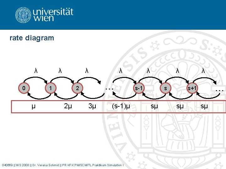
rate diagram λ 0 λ λ 1 μ λ … 2 2μ 3μ (s-1)μ 040669 || WS 2008 || Dr. Verena Schmid || PR KFK PM/SCM/TL Praktikum Simulation I λ λ s-1 s sμ λ … s+1 sμ sμ

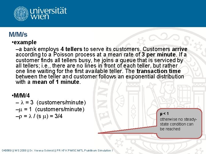
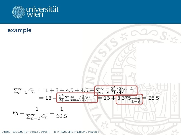
M/M/s • example –a bank employs 4 tellers to serve its customers. Customers arrive according to a Poisson process at a mean rate of 3 per minute. If a customer finds all tellers busy, he joins a queue that is serviced by all tellers; i. e. , there are no lines in front of each teller, but rather one line waiting for the first available teller. The transaction time between the teller and customer follows an exponential distribution with a mean of 1 minute. • M/M/4 – = 3 (customers/minute) – = 1 (customers/minute) – = / (s ) = 3/4 040669 || WS 2008 || Dr. Verena Schmid || PR KFK PM/SCM/TL Praktikum Simulation I <1 otherwise no steadystate condition can be reached

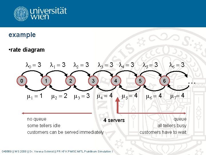
example • rate diagram 0 = 3 0 1 = 3 1 1 = 1 2 2 = 2 3 = 3 4 = 3 2 = 3 3 3 = 3 4 4 = 4 5 5 = 4 no queue 4 servers some tellers idle customers can be served immediately 040669 || WS 2008 || Dr. Verena Schmid || PR KFK PM/SCM/TL Praktikum Simulation I 5 = 3 6 = 3 … 6 6 = 4 7= 4 queue all tellers busy customers have to wait

example 040669 || WS 2008 || Dr. Verena Schmid || PR KFK PM/SCM/TL Praktikum Simulation I

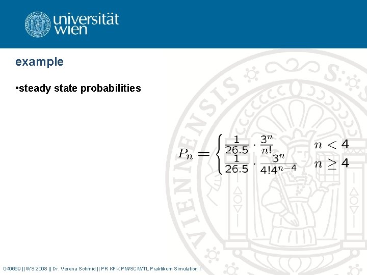
example • steady state probabilities 040669 || WS 2008 || Dr. Verena Schmid || PR KFK PM/SCM/TL Praktikum Simulation I

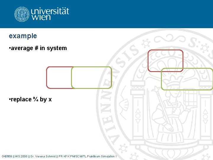
example • average # in system • replace ¾ by x 040669 || WS 2008 || Dr. Verena Schmid || PR KFK PM/SCM/TL Praktikum Simulation I

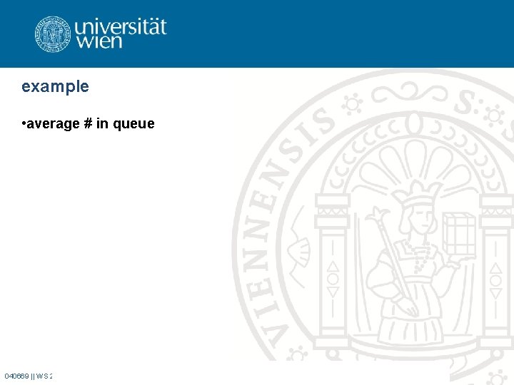
example • average # in queue 040669 || WS 2008 || Dr. Verena Schmid || PR KFK PM/SCM/TL Praktikum Simulation I

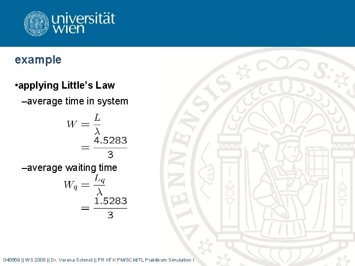
example • applying Little’s Law –average time in system –average waiting time 040669 || WS 2008 || Dr. Verena Schmid || PR KFK PM/SCM/TL Praktikum Simulation I

formulas for M/M/s 040669 || WS 2008 || Dr. Verena Schmid || PR KFK PM/SCM/TL Praktikum Simulation I

formulas for M/M/s 040669 || WS 2008 || Dr. Verena Schmid || PR KFK PM/SCM/TL Praktikum Simulation I

M/M/s/K finite queue variation of the M/M/s

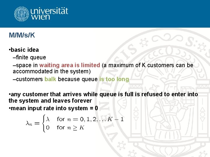
M/M/s/K • basic idea –finite queue –space in waiting area is limited (a maximum of K customers can be accommodated in the system) –customers balk because queue is too long • any customer that arrives while queue is full is refused to enter into the system and leaves forever • mean input rate into system = 0

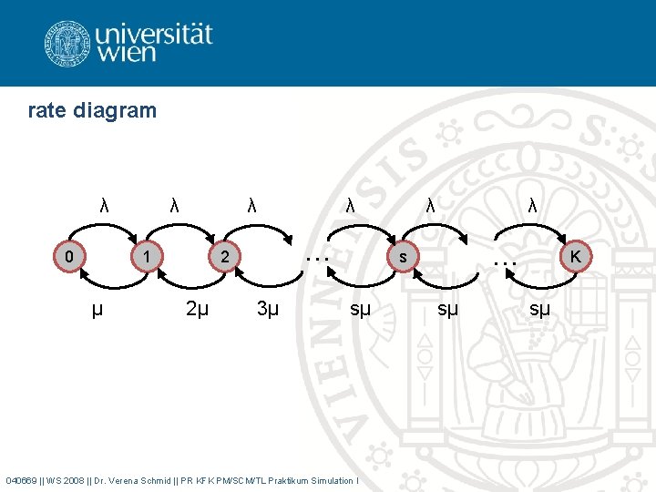
rate diagram λ 0 λ λ 1 μ λ … 2 2μ 3μ λ λ … s sμ 040669 || WS 2008 || Dr. Verena Schmid || PR KFK PM/SCM/TL Praktikum Simulation I sμ K sμ

M/M/s/K • example –an airline ticket office as two ticket agents answering incoming phone calls for flight reservations. In addition, one caller can be put on hold until one the agents is available to take the call. –If all three phone lines (both agent lines and the hold line) are busy, a potential customer gets a busy signal, and it’s assumed that the call goes to another ticket office and that the business is lost. –The calls and attempted calls occur randomly (i. e. according to a Poisson process) at a mean rate of 15 per hour. The length of a telephone conversation has an exponential distribution with a mean of 4 minutes. –M/M/2/3 – = 15 (per hour) 040669 || WS 2008 || Dr. Verena Schmid || PR KFK PM/SCM/TL Praktikum Simulation I

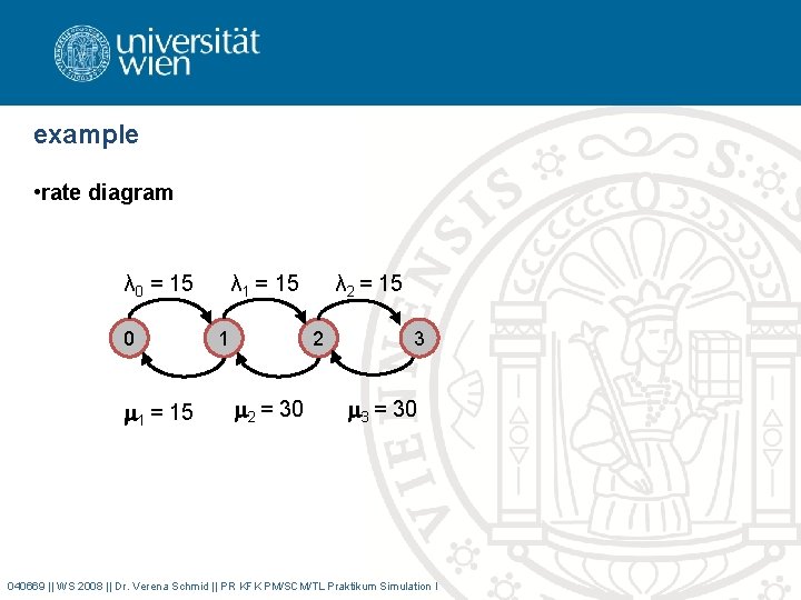
example • rate diagram λ 0 = 15 0 1 = 15 λ 1 = 15 1 λ 2 = 15 2 2 = 30 3 3 = 30 040669 || WS 2008 || Dr. Verena Schmid || PR KFK PM/SCM/TL Praktikum Simulation I

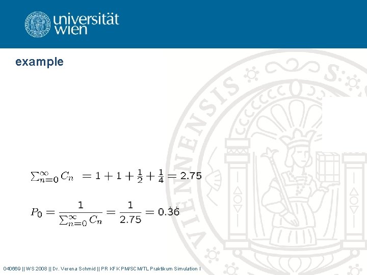
example 040669 || WS 2008 || Dr. Verena Schmid || PR KFK PM/SCM/TL Praktikum Simulation I

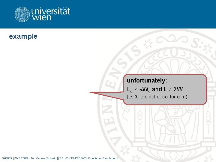
example unfortunately: Lq Wq and L W (as n are not equal for all n) 040669 || WS 2008 || Dr. Verena Schmid || PR KFK PM/SCM/TL Praktikum Simulation I

formulas for M/M/s/K 040669 || WS 2008 || Dr. Verena Schmid || PR KFK PM/SCM/TL Praktikum Simulation I

formulas for M/M/s/K 040669 || WS 2008 || Dr. Verena Schmid || PR KFK PM/SCM/TL Praktikum Simulation I

finite calling population variation of M/M/s

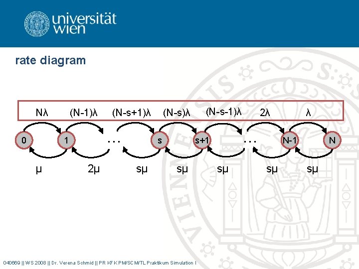
M/M/s with finite calling population • basic idea –input source is limited –size of calling population is finite (N) –if there’re n customers in the queuing system only N-n potential customers remain in the input source • example: machine repair problem –maintenance person (servers) –responsible to repair machines (customers) in case of breakdowns –arrival: machine breaks down –service-time: time required for repair –departure: machine is working again 040669 || WS 2008 || Dr. Verena Schmid || PR KFK PM/SCM/TL Praktikum Simulation I

rate diagram Nλ 0 (N-1)λ … 1 μ (N-s+1)λ 2μ s sμ (N-s-1)λ (N-s)λ … s+1 sμ 040669 || WS 2008 || Dr. Verena Schmid || PR KFK PM/SCM/TL Praktikum Simulation I 2λ sμ λ N-1 sμ N sμ

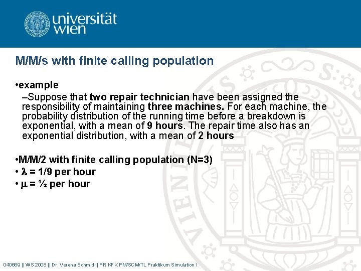
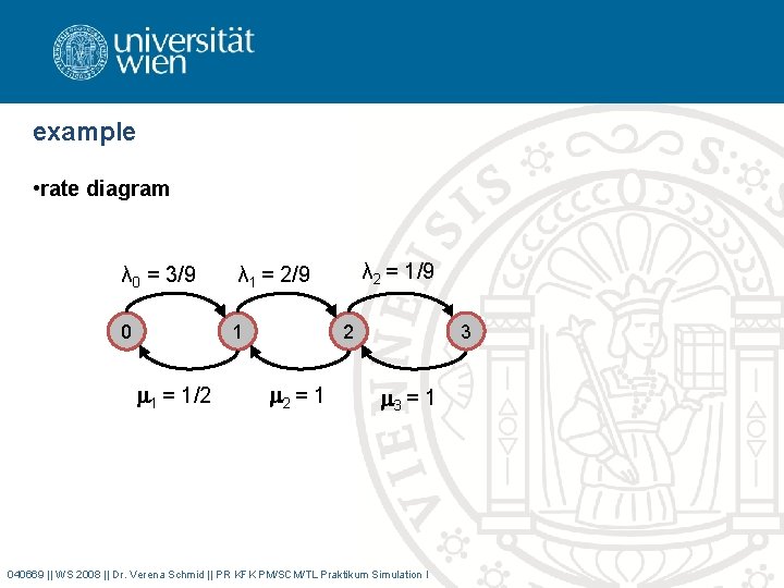
M/M/s with finite calling population • example –Suppose that two repair technician have been assigned the responsibility of maintaining three machines. For each machine, the probability distribution of the running time before a breakdown is exponential, with a mean of 9 hours. The repair time also has an exponential distribution, with a mean of 2 hours • M/M/2 with finite calling population (N=3) • = 1/9 per hour • = ½ per hour 040669 || WS 2008 || Dr. Verena Schmid || PR KFK PM/SCM/TL Praktikum Simulation I

example • rate diagram λ 0 = 3/9 0 1 1 = 1/2 λ 2 = 1/9 λ 1 = 2/9 3 2 2 = 1 3 = 1 040669 || WS 2008 || Dr. Verena Schmid || PR KFK PM/SCM/TL Praktikum Simulation I

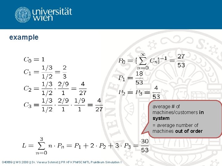
example average # of machines/customers in system = average number of machines out of order 040669 || WS 2008 || Dr. Verena Schmid || PR KFK PM/SCM/TL Praktikum Simulation I

formulas for M/M/s with finite calling population 040669 || WS 2008 || Dr. Verena Schmid || PR KFK PM/SCM/TL Praktikum Simulation I

formulas for M/M/s with finite calling population 040669 || WS 2008 || Dr. Verena Schmid || PR KFK PM/SCM/TL Praktikum Simulation I

extensions

M/Ek/s • total service required might be more than one single task ! rather a sequence of k tasks • if single tasks have an identical exponential distribution for their duration ! total service time will have an Erlang distribution • remember –T 1, T 2, …, Tk k independent random variables with an identical exponential distribution (mean = 1/(k ) ) –their sum has an Erlang distribution with parameters k and 040669 || WS 2008 || Dr. Verena Schmid || PR KFK PM/SCM/TL Praktikum Simulation I

further extensions • state-dependent service rates and/or arrival rates • queuing models involving nonexponential distributions and/or without Poisson input • priority-discipline queuing models –nonpreemtive vs. preemtive • queuing networks • etc. 040669 || WS 2008 || Dr. Verena Schmid || PR KFK PM/SCM/TL Praktikum Simulation I