Queueing Theory Delay Models MM1 queueing system n
")

![M/M/1 queueing system P[1 arrival and no departure in δ]= where the arrival and](https://slidetodoc.com/presentation_image/2b40a0860a95425324f3186c8a801f0a/image-3.jpg "M/M/1 queueing system P[1 arrival and no departure in δ]= where the arrival and")


 by")


 l l l (a) Average number of messages in")
![M/M/1 Example I (cont. ) 1. 2. 3. 4. E[s] = Average Message Length](https://slidetodoc.com/presentation_image/2b40a0860a95425324f3186c8a801f0a/image-19.jpg "M/M/1 Example I (cont. ) 1. 2. 3. 4. E[s] = Average Message Length")
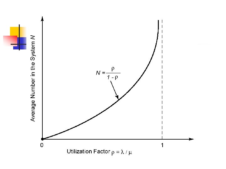
 l l l (a) N= r / (1 -")

 mean of 30 minutes. The branch office receives complains")
 1. {10 person / day}×{1 day / 8 hr}×{1")
 l l l Arrival Rate = 1 / 48")
 l l l Mean time a customer spends in")
 Mean time in queue for those who must wait")
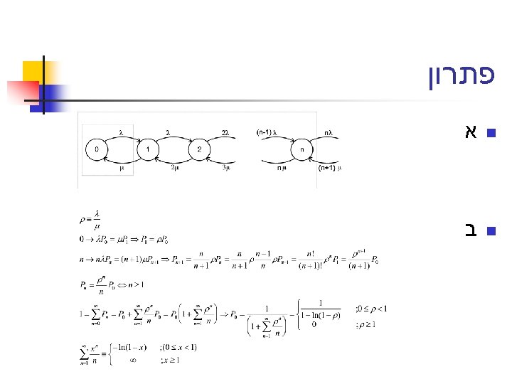
 n detailed balance equations in steady state")


 = 0. 429 (@ 43% of time, system")
 n Find W Wq = Lq / =")


")


- Slides: 40
Queueing Theory (Delay Models)
M/M/1 queueing system n Arrival statistics: stochastic process taking nonnegative integer values is called a Poisson process with rate λ if n n n A(t) is a counting process representing the total number of arrivals from 0 to t arrivals are independent probability distribution function
M/M/1 queueing system P[1 arrival and no departure in δ]= where the arrival and departure processes are independent
M/M/1 queueing system n Global balance equation
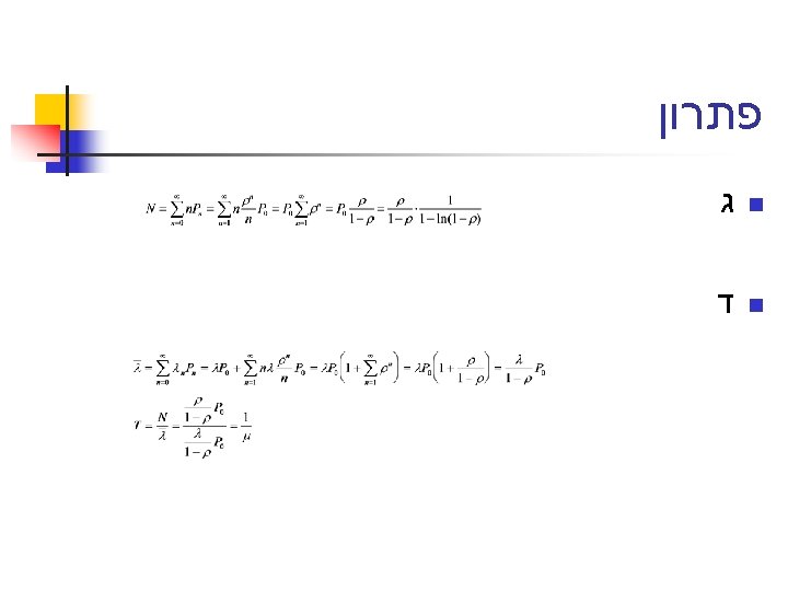
M/M/1 queueing system from Then n Average number of customers in the system
M/M/1 queueing system n Average delay per customer (waiting time + service time) by Little’s theorem Average waiting time n Average number of customer in queue n Server utilization n
M/M/1 queueing system n example 1/λ=4 ms, 1/μ=3 ms
פתרון Arrival rate: =1/K Time in the system: T= K+P Applying Little’s theorem: N= T = +P/K Though the process is deterministic, and N(t) does not converge to any value, N is well defined, interpreted as the time average
פתרון א Message Length: Transmission Rate: Transmission Time: Service Rate:
M/M/1 Example I Traffic to a message switching center for one of the outgoing communication lines arrive in a random pattern at an average rate of 240 messages per minute. The line has a transmission rate of 800 characters per second. The message length distribution (including control characters) is approximately exponential with an average length of 176 characters. Calculate the following principal statistical measures of system performance, assuming that a very large number of message buffers are provided: Queueing Theory 41
M/M/1 Example I (cont. ) l l l (a) Average number of messages in the system (b) Average number of messages in the queue waiting to be transmitted. (c) Average time a message spends in the system. (d) Average time a message waits for transmission (e) Probability that 10 or more messages are waiting to be transmitted. Queueing Theory 42
M/M/1 Example I (cont. ) 1. 2. 3. 4. E[s] = Average Message Length / Line Speed = {176 char/message} / {800 char/sec} = 0. 22 sec/message or = 1 / 0. 22 {message / sec} = 4. 55 message / sec = 240 message / min = 4 message / sec r = E[s] = / = 0. 88 Queueing Theory 43
M/M/1 Example I (cont. ) l l l (a) N= r / (1 - r) = 7. 33 (messages) (b) Nq = r 2 / (1 - r) = 6. 45 (messages) (c) W = E[s] / (1 - r) = 1. 83 (sec) (d) Wq = r × E[s] / (1 - r) = 1. 61 (sec) (e) P [11 or more messages in the system] = r 11 = 0. 245 Queueing Theory 44
M/M/1 Example II A branch office of a large engineering firm has one on -line terminal that is connected to a central computer system during the normal eight-hour working day. Engineers, who work throughout the city, drive to the branch office to use the terminal to make routine calculations. Statistics collected over a period of time indicate that the arrival pattern of people at the branch office to use the terminal has a Poisson (random) distribution, with a mean of 10 people coming to use the terminal each day. The distribution of time spent by an engineer at a terminal is exponential, with a Queueing Theory 45
M/M/1 Example II (cont. ) mean of 30 minutes. The branch office receives complains from the staff about the terminal service. It is reported that individuals often wait over an hour to use the terminal and it rarely takes less than an hour and a half in the office to complete a few calculations. The manager is puzzled because the statistics show that the terminal is in use only 5 hours out of 8, on the average. This level of utilization would not seem to justify the acquisition of another terminal. What insight can queueing theory provide? Queueing Theory 46
M/M/1 Example II (cont. ) 1. {10 person / day}×{1 day / 8 hr}×{1 hr / 60 min} 1. = 10 person / 480 min = 1 person / 48 min ==> = 1 / 48 (person / min) 30 minutes : 1 person = 1 (min) : 1/30 (person) ==> = 1 / 30 (person / min) r = / = {1/48} / {1/30} = 30 / 48 =5/8 Queueing Theory 2. 47
M/M/1 Example II (cont. ) l l l Arrival Rate = 1 / 48 (customer / min) Server Utilization r = / = 5 / 8 = 0. 625 Probability of 2 or more customers in system P[N ³ 2] = r 2 = 0. 391 Mean steady-state number in the system L = E[N] = r / (1 - r) = 1. 667 S. D. of number of customers in the system s. N = sqrt(r) / (1 - r) = 2. 108 Queueing Theory 48
M/M/1 Example II (cont. ) l l l Mean time a customer spends in the system W = E[w] = E[s] / (1 - r) = 80 (min) S. D. of time a customer spends in the system sw = E[w] = 80 (min) Mean steady-state number of customers in queue Nq = r 2 / (1 - r) = 1. 04 Mean steady-state queue length of nonempty Qs E[Nq | Nq > 0] = 1 / (1 - r) = 2. 67 Mean time in queue Wq = E[q] = r×E[s] / (1 - r) = 50 (min) Queueing Theory 49
M/M/1 Example II (cont. ) Mean time in queue for those who must wait E[q | q > 0] = E[w] = 80 (min) 90 th percentile of the time in queue pq(90) = E[w] ln (10 r) = 80 * 1. 8326 = 146. 6 (min) Queueing Theory l l 50
M/M/m, M/M/m/m, M/M/∞ n M/M/m (infinite buffer) n detailed balance equations in steady state
M/M/m where From
M/M/m n The probability that all servers are busy - Erlang C formula n expected number of customers waiting in queue
M/M/m n average waiting time of a customer in queue n average delay per customer n average number of customer in the system by Little’s theorem
M/M/s Case Example I Find p 0 Queueing Theory 55
M/M/s Case Example I (cont. ) = 0. 429 (@ 43% of time, system is empty) as compared to m = 1: P 0 = 0. 20 Queueing Theory 56
M/M/s Case Example I (cont. ) n Find W Wq = Lq / = 0. 152 / (1/10) = 1. 52 (min) W = Wq + 1 / = 1. 52 + 1 / (1/8) = 9. 52 min) n What proportion of time is both repairman busy? (long run) P(N ³ 2) = 1 - P 0 - P 1 = 1 - 0. 429 - 0. 343 = 0. 228 (Good or Bad? ) n Queueing Theory 57
M/M/∞ n M/M/∞: The infinite server case n The detailed balance equations Then
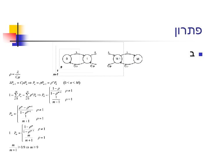
M/M/m/m n M/M/m/m : The m server loss system n n when m servers are busy, next arrival will be lost circuit switched network model
M/M/m/m n The blocking probability (Erlang-B formula)
Moment Generating Function
Discrete Random Variables
Continuous Random Variables